library(sf)Linking to GEOS 3.10.2, GDAL 3.4.1, PROJ 8.2.1; sf_use_s2() is TRUElibrary(stars)Loading required package: abindlibrary(mapview)Part 1: Extracting to points
First we load the main R packages for working with spatial data:
we also load the mapview package for interactive visualization. Therefore:
library(sf)Linking to GEOS 3.10.2, GDAL 3.4.1, PROJ 8.2.1; sf_use_s2() is TRUElibrary(stars)Loading required package: abindlibrary(mapview)To import a vector layer into the R environment, we use the sf::st_read function:
pnt = st_read('data/export/Address coordinates.gpkg')Reading layer `extracted' from data source
`/home/michael/Sync/presentations/p_2023_01_R_exposure_tutorial/data/export/Address coordinates.gpkg'
using driver `GPKG'
Simple feature collection with 13710 features and 2 fields
Geometry type: POINT
Dimension: XY
Bounding box: xmin: 669825 ymin: 6578850 xmax: 695023 ymax: 6590699
Projected CRS: SWEREF99 TMThe result is an sf object:
pntSimple feature collection with 13710 features and 2 fields
Geometry type: POINT
Dimension: XY
Bounding box: xmin: 669825 ymin: 6578850 xmax: 695023 ymax: 6590699
Projected CRS: SWEREF99 TM
First 10 features:
X_sw99_corr_final Y_sw99_corr_final geom
1 6579476 672969 POINT (672969 6579476)
2 6579535 672998 POINT (672998 6579535)
3 6580754 673589 POINT (673589 6580754)
4 6580685 670730 POINT (670730 6580685)
5 6580685 670730 POINT (670730 6580685)
6 6580707 670681 POINT (670681 6580707)
7 6580685 670730 POINT (670730 6580685)
8 6580063 671015 POINT (671015 6580063)
9 6581347 672437 POINT (672437 6581347)
10 6582407 673401 POINT (673401 6582407)The sf class extends the data.frame class. A vector layer is basically a data.frame where one of the columns contains geometries (Figure 1).
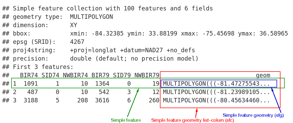
sf object (from https://r-spatial.github.io/sf/articles/sf1.html)plot(st_geometry(pnt))
We also import the polygons layer:
pol = st_read('data/export/Noise/Railway noise/Heay railways Stockholm/END/Buller_Jvg_2017_Lden/Buller_Jvg_2017_Lden.shp')Reading layer `Buller_Jvg_2017_Lden' from data source
`/home/michael/Sync/presentations/p_2023_01_R_exposure_tutorial/data/export/Noise/Railway noise/Heay railways Stockholm/END/Buller_Jvg_2017_Lden/Buller_Jvg_2017_Lden.shp'
using driver `ESRI Shapefile'
Simple feature collection with 14 features and 5 fields
Geometry type: MULTIPOLYGON
Dimension: XY
Bounding box: xmin: 669800 ymin: 6578800 xmax: 675618.7 ymax: 6588767
Projected CRS: SWEREF99 TMpolSimple feature collection with 14 features and 5 fields
Geometry type: MULTIPOLYGON
Dimension: XY
Bounding box: xmin: 669800 ymin: 6578800 xmax: 675618.7 ymax: 6588767
Projected CRS: SWEREF99 TM
First 10 features:
KOMMUNNAMN CTRYID RepEntUnCD DB_LOW DB_HIGH geometry
1 Sollentuna SE a 50 55 MULTIPOLYGON (((669800.8 65...
2 Sollentuna SE a 55 60 MULTIPOLYGON (((669810 6588...
3 Solna SE a 50 55 MULTIPOLYGON (((669801.2 65...
4 Solna SE a 55 60 MULTIPOLYGON (((669810 6583...
5 Solna SE a 60 65 MULTIPOLYGON (((669810 6583...
6 Solna SE a 65 70 MULTIPOLYGON (((669810 6583...
7 Solna SE a 70 75 MULTIPOLYGON (((671880 6582...
8 Solna SE a 75 75 MULTIPOLYGON (((671325 6583...
9 Stockholm SE a 50 55 MULTIPOLYGON (((671484.1 65...
10 Stockholm SE a 55 60 MULTIPOLYGON (((672006 6581...plot(pol)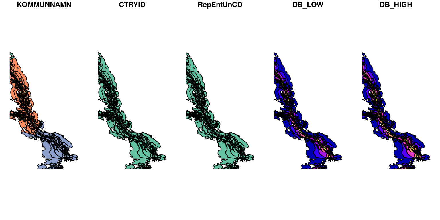
plot(pol['DB_HIGH'])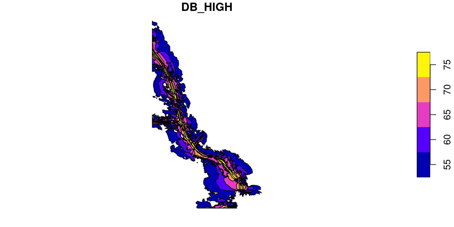
To plot more than one layer at once, we use add=TRUE in any subsequent plot calls:
plot(st_geometry(pnt), col = 'grey', axes = TRUE)
plot(st_geometry(pol), add = TRUE)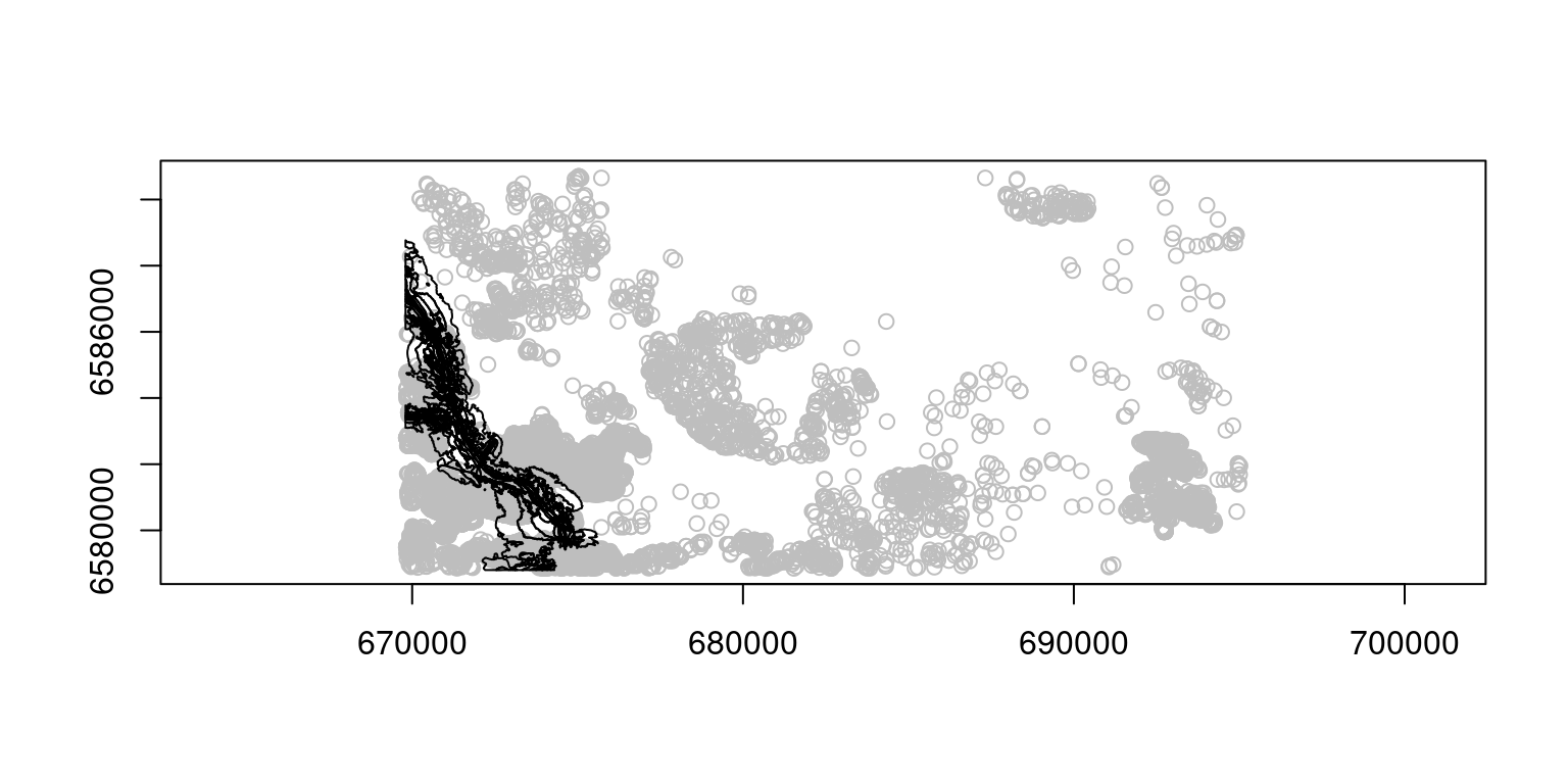
To import a raster into the R environment, we use the stars::read_stars function. The result is a stars object:
r = read_stars('data/export/Greenness/NDVI/WholeSwedenNAv2017.tif')The stars class is basically an extended array, where the axes (typically x+y, or x+y+band) are labeled and associated with metadata:
rstars object with 2 dimensions and 1 attribute
attribute(s):
Min. 1st Qu. Median Mean 3rd Qu. Max. NA's
WholeSwedenNAv2017.tif 64 507 628 572.7616 695 855 151241
dimension(s):
from to offset delta refsys point values x/y
x 1 1012 669800 25 SWEREF99 TM FALSE NULL [x]
y 1 476 6590700 -25 SWEREF99 TM FALSE NULL [y]It is convenient to rename the raster attribute to a meaningful name (otherwise the defailt is the file name, e.g., WholeSwedenNAv2017.tif):
names(r) = 'ndvi'
rstars object with 2 dimensions and 1 attribute
attribute(s):
Min. 1st Qu. Median Mean 3rd Qu. Max. NA's
ndvi 64 507 628 572.7616 695 855 151241
dimension(s):
from to offset delta refsys point values x/y
x 1 1012 669800 25 SWEREF99 TM FALSE NULL [x]
y 1 476 6590700 -25 SWEREF99 TM FALSE NULL [y]plot(r)
We can plot the three layers together, to make sure they are aligned:
plot(r, col = hcl.colors(11, 'Spectral'), axes = TRUE, reset = FALSE)
plot(st_geometry(pnt), add = TRUE)
plot(st_geometry(pol), col = 'yellow', add = TRUE)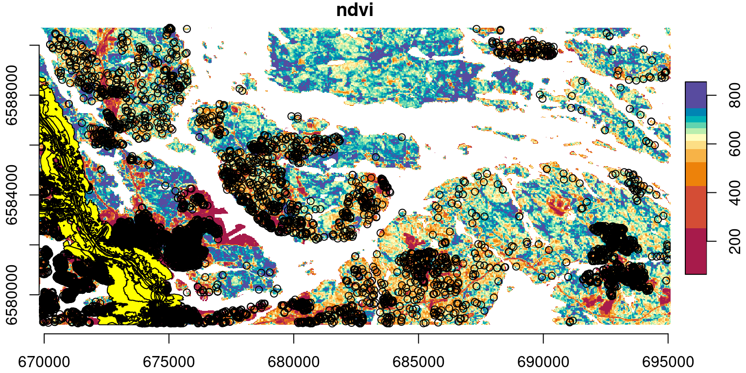
The mapview package can be used for interactively examining spatial layers in R, with basemaps, for context, and “identify” capabilities. For example:
mapview(r) + mapview(pol, zcol = 'DB_HIGH') + mapview(pnt)To extract polygon values to points, we do a spatial join, using the st_join function. The defaults of additional parameters are appropriate for our use case:
join=st_intersects—Join based on “intersects” spatial relationleft=TRUE—A left joinTherefore:
pnt = st_join(pnt, pol)As a result, the pnt layer has new attributes joined from coinciding pol features, namely KOMMUNNAMN, CTRYID, RepEntUnCD, DB_LOW, and DB_HIGH. Note that there are missing values where no match was found:
pntSimple feature collection with 13710 features and 7 fields
Geometry type: POINT
Dimension: XY
Bounding box: xmin: 669825 ymin: 6578850 xmax: 695023 ymax: 6590699
Projected CRS: SWEREF99 TM
First 10 features:
X_sw99_corr_final Y_sw99_corr_final KOMMUNNAMN CTRYID RepEntUnCD DB_LOW
1 6579476 672969 Stockholm SE a 50
2 6579535 672998 Stockholm SE a 50
3 6580754 673589 Stockholm SE a 60
4 6580685 670730 <NA> <NA> <NA> NA
5 6580685 670730 <NA> <NA> <NA> NA
6 6580707 670681 <NA> <NA> <NA> NA
7 6580685 670730 <NA> <NA> <NA> NA
8 6580063 671015 <NA> <NA> <NA> NA
9 6581347 672437 Stockholm SE a 50
10 6582407 673401 <NA> <NA> <NA> NA
DB_HIGH geom
1 55 POINT (672969 6579476)
2 55 POINT (672998 6579535)
3 65 POINT (673589 6580754)
4 NA POINT (670730 6580685)
5 NA POINT (670730 6580685)
6 NA POINT (670681 6580707)
7 NA POINT (670730 6580685)
8 NA POINT (671015 6580063)
9 55 POINT (672437 6581347)
10 NA POINT (673401 6582407)We can plot, for example, the DB_HIGH values (with all point locations in grey):
plot(st_geometry(pnt), col = 'grey')
plot(pnt['DB_HIGH'], add = TRUE)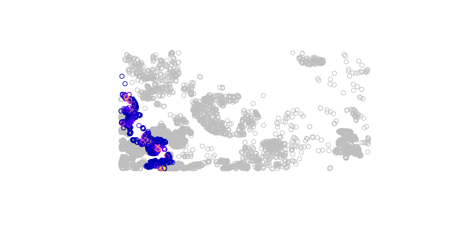
To extract raster values to points, we use the st_extract function. The result is a new sf layer, with the point geometries and the extracted raster attribute(s):
x = st_extract(r, pnt)
xSimple feature collection with 13710 features and 1 field
Geometry type: POINT
Dimension: XY
Bounding box: xmin: 669825 ymin: 6578850 xmax: 695023 ymax: 6590699
Projected CRS: SWEREF99 TM
First 10 features:
ndvi geom
1 143 POINT (672969 6579476)
2 167 POINT (672998 6579535)
3 245 POINT (673589 6580754)
4 158 POINT (670730 6580685)
5 158 POINT (670730 6580685)
6 238 POINT (670681 6580707)
7 158 POINT (670730 6580685)
8 231 POINT (671015 6580063)
9 173 POINT (672437 6581347)
10 280 POINT (673401 6582407)It is typically more useful to attach the extracted values to the original point layer:
pnt$ndvi = x$ndvi
pntSimple feature collection with 13710 features and 8 fields
Geometry type: POINT
Dimension: XY
Bounding box: xmin: 669825 ymin: 6578850 xmax: 695023 ymax: 6590699
Projected CRS: SWEREF99 TM
First 10 features:
X_sw99_corr_final Y_sw99_corr_final KOMMUNNAMN CTRYID RepEntUnCD DB_LOW
1 6579476 672969 Stockholm SE a 50
2 6579535 672998 Stockholm SE a 50
3 6580754 673589 Stockholm SE a 60
4 6580685 670730 <NA> <NA> <NA> NA
5 6580685 670730 <NA> <NA> <NA> NA
6 6580707 670681 <NA> <NA> <NA> NA
7 6580685 670730 <NA> <NA> <NA> NA
8 6580063 671015 <NA> <NA> <NA> NA
9 6581347 672437 Stockholm SE a 50
10 6582407 673401 <NA> <NA> <NA> NA
DB_HIGH geom ndvi
1 55 POINT (672969 6579476) 143
2 55 POINT (672998 6579535) 167
3 65 POINT (673589 6580754) 245
4 NA POINT (670730 6580685) 158
5 NA POINT (670730 6580685) 158
6 NA POINT (670681 6580707) 238
7 NA POINT (670730 6580685) 158
8 NA POINT (671015 6580063) 231
9 55 POINT (672437 6581347) 173
10 NA POINT (673401 6582407) 280The same can be done in one step, as follows:
pnt$ndvi = st_extract(r, pnt)$ndvi
pntSimple feature collection with 13710 features and 8 fields
Geometry type: POINT
Dimension: XY
Bounding box: xmin: 669825 ymin: 6578850 xmax: 695023 ymax: 6590699
Projected CRS: SWEREF99 TM
First 10 features:
X_sw99_corr_final Y_sw99_corr_final KOMMUNNAMN CTRYID RepEntUnCD DB_LOW
1 6579476 672969 Stockholm SE a 50
2 6579535 672998 Stockholm SE a 50
3 6580754 673589 Stockholm SE a 60
4 6580685 670730 <NA> <NA> <NA> NA
5 6580685 670730 <NA> <NA> <NA> NA
6 6580707 670681 <NA> <NA> <NA> NA
7 6580685 670730 <NA> <NA> <NA> NA
8 6580063 671015 <NA> <NA> <NA> NA
9 6581347 672437 Stockholm SE a 50
10 6582407 673401 <NA> <NA> <NA> NA
DB_HIGH geom ndvi
1 55 POINT (672969 6579476) 143
2 55 POINT (672998 6579535) 167
3 65 POINT (673589 6580754) 245
4 NA POINT (670730 6580685) 158
5 NA POINT (670730 6580685) 158
6 NA POINT (670681 6580707) 238
7 NA POINT (670730 6580685) 158
8 NA POINT (671015 6580063) 231
9 55 POINT (672437 6581347) 173
10 NA POINT (673401 6582407) 280plot(pnt['ndvi'])To export an sf object from the R environment into a vector layer file, we use the sf::st_write function.
.shp, .gpkg, .geojson)delete_dsn=TRUE—Delete an existing file, if there is any (i.e., overwrites)layer_options="ENCODING=..." (e.g., layer_options="ENCODING=UTF-8")—can be used to specify the encodingFor example, here is how we export pnt with the extracted attributes to a GeoPackage file named pnt1.gpkg:
st_write(pnt, 'pnt1.gpkg', delete_dsn = TRUE)Deleting source `pnt1.gpkg' using driver `GPKG'
Writing layer `pnt1' to data source `pnt1.gpkg' using driver `GPKG'
Writing 13710 features with 8 fields and geometry type Point.The exported file can be opened in QGIS (Figure 8), or any other software for working with vector layers.
