Linking exposures to residential adresses

Part 2: Extracting to buffers

Authors

Michael Dorman

Itai Kloog

Published

January 19, 2023

Download R script

Download data

Setup

We load sf and stars, and also terra which will be needed for extracting raster values to polygons.

library(sf)

Linking to GEOS 3.10.2, GDAL 3.4.1, PROJ 8.2.1; sf_use_s2() is TRUE

library(stars)

Loading required package: abind

library(terra)

terra 1.6.7

Input data

Points

Importing the points:

pnt = st_read('data/export/Address coordinates.gpkg')

Reading layer `extracted' from data source 
  `/home/michael/Sync/presentations/p_2023_01_R_exposure_tutorial/data/export/Address coordinates.gpkg' 
  using driver `GPKG'
Simple feature collection with 13710 features and 2 fields
Geometry type: POINT
Dimension:     XY
Bounding box:  xmin: 669825 ymin: 6578850 xmax: 695023 ymax: 6590699
Projected CRS: SWEREF99 TM

pnt

Simple feature collection with 13710 features and 2 fields
Geometry type: POINT
Dimension:     XY
Bounding box:  xmin: 669825 ymin: 6578850 xmax: 695023 ymax: 6590699
Projected CRS: SWEREF99 TM
First 10 features:
   X_sw99_corr_final Y_sw99_corr_final                   geom
1            6579476            672969 POINT (672969 6579476)
2            6579535            672998 POINT (672998 6579535)
3            6580754            673589 POINT (673589 6580754)
4            6580685            670730 POINT (670730 6580685)
5            6580685            670730 POINT (670730 6580685)
6            6580707            670681 POINT (670681 6580707)
7            6580685            670730 POINT (670730 6580685)
8            6580063            671015 POINT (671015 6580063)
9            6581347            672437 POINT (672437 6581347)
10           6582407            673401 POINT (673401 6582407)

plot(st_geometry(pnt))

Raster

Importing the raster:

r = read_stars('data/export/Greenness/NDVI/WholeSwedenNAv2017.tif')
names(r) = 'ndvi'
r

stars object with 2 dimensions and 1 attribute
attribute(s):
      Min. 1st Qu. Median     Mean 3rd Qu. Max.   NA's
ndvi    64     507    628 572.7616     695  855 151241
dimension(s):
  from   to  offset delta      refsys point values x/y
x    1 1012  669800    25 SWEREF99 TM FALSE   NULL [x]
y    1  476 6590700   -25 SWEREF99 TM FALSE   NULL [y]

plot(r)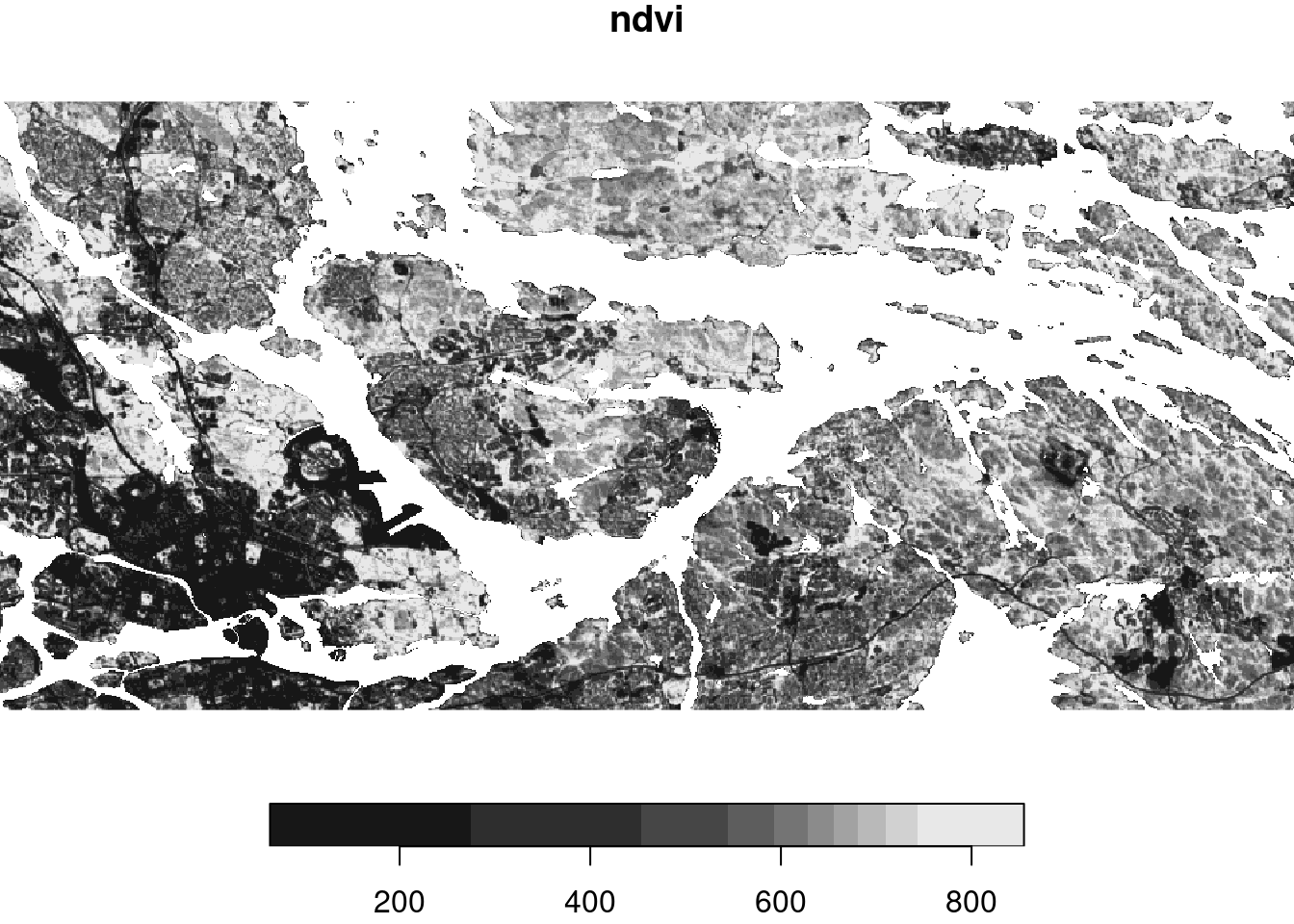

Creating buffers

The st_buffer function is used to create buffers, with specified width (in CRS units). For example, here is how we can create 100, 250, and 500 \(m\) buffer layers, named pol_100, pol_250, and pol_500, respectively:

pol_100 = st_buffer(pnt, 100)
pol_250 = st_buffer(pnt, 250)
pol_500 = st_buffer(pnt, 500)

Confirming that the CRS units are indeed \(m\) can be done as follows:

st_crs(pnt)$units

[1] "m"

Each of the layers pol_100, pol_250, and pol_500 is identical to the input pnt, only that the POINT geometries were replaced with POLYGON geometries of the respective buffers. For example:

pol_500

Simple feature collection with 13710 features and 2 fields
Geometry type: POLYGON
Dimension:     XY
Bounding box:  xmin: 669325 ymin: 6578350 xmax: 695523 ymax: 6591199
Projected CRS: SWEREF99 TM
First 10 features:
   X_sw99_corr_final Y_sw99_corr_final                           geom
1            6579476            672969 POLYGON ((673469 6579476, 6...
2            6579535            672998 POLYGON ((673498 6579535, 6...
3            6580754            673589 POLYGON ((674089 6580754, 6...
4            6580685            670730 POLYGON ((671230 6580685, 6...
5            6580685            670730 POLYGON ((671230 6580685, 6...
6            6580707            670681 POLYGON ((671181 6580707, 6...
7            6580685            670730 POLYGON ((671230 6580685, 6...
8            6580063            671015 POLYGON ((671515 6580063, 6...
9            6581347            672437 POLYGON ((672937 6581347, 6...
10           6582407            673401 POLYGON ((673901 6582407, 6...

Figure 3 shows the 500-\(m\) buffers:

plot(st_geometry(pol_500))

and Figure 4 shows all three (100, 250, and 500 \(m\)) buffers for one point:

plot(st_geometry(pnt[1, ]), pch = 3, extent = st_bbox(pol_500[1, ]))
plot(st_geometry(pol_500[1, ]), border = 'red', add = TRUE)
plot(st_geometry(pol_250[1, ]), border = 'green', add = TRUE)
plot(st_geometry(pol_100[1, ]), border = 'blue', add = TRUE)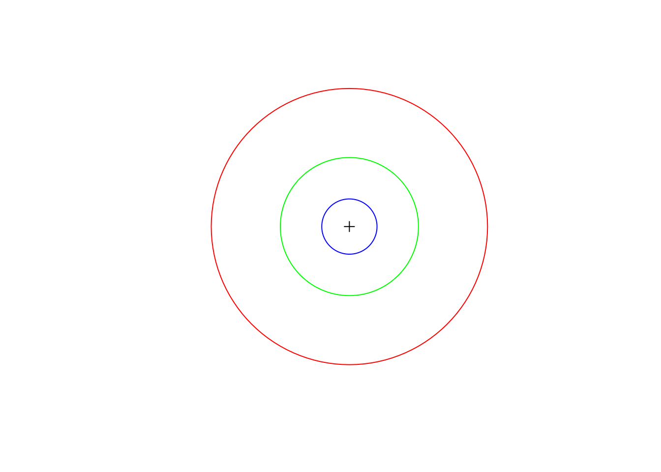

Extracting raster values to polygons—`stars`

Extracting raster values to polygons in the sf+stars framework can be done using function aggregate, similarly to the base method for data.frame. For example, to calculate the median r value in each pol_100 buffer excluding NA, we use:

x = aggregate(r, pol_100, median, na.rm = TRUE)
x = st_as_sf(x)
x

Simple feature collection with 13710 features and 1 field
Geometry type: POLYGON
Dimension:     XY
Bounding box:  xmin: 669725 ymin: 6578750 xmax: 695123 ymax: 6590799
Projected CRS: SWEREF99 TM
First 10 features:
    ndvi                           geom
1  292.5 POLYGON ((673069 6579476, 6...
2  268.0 POLYGON ((673098 6579535, 6...
3  202.0 POLYGON ((673689 6580754, 6...
4  304.0 POLYGON ((670830 6580685, 6...
5     NA POLYGON ((670830 6580685, 6...
6  355.0 POLYGON ((670781 6580707, 6...
7     NA POLYGON ((670830 6580685, 6...
8  295.0 POLYGON ((671115 6580063, 6...
9  118.0 POLYGON ((672537 6581347, 6...
10 186.0 POLYGON ((673501 6582407, 6...

However (!), probably for compatibility with other aggregate methods in R, each pixel can only be assigned into one grouping polygon. Therefore overlapping polygons capture the values of “unassigned” pixels only:

aggregate(r, pol_100[rep(1,3), ], median, na.rm = TRUE)[[1]]

[1] 292.5    NA    NA

This means that aggregate works incorrectly for any polygon layer that has overlapping polygons, such as our buffer layers (Figure 3).

Extracting raster values to polygons—`terra`

The terra package provides another framework for working with rasters in R. There is very large overlap in functionality between stars and terra, with few exceptions. For example, terra has an extract function for summarizing raster values per polygons, without the above-mentioned issue that aggregate has.

The terra package has its own classes for rasters and vector layers. Before using terra::extract we therefore need to transform our objects to the terra classes:

Rasters—stars→SpatRaster, using function rast
Vector layers—sf→SpatVector, using function vect

For example:

pol_100_t = vect(pol_100)
pol_100_t

 class       : SpatVector 
 geometry    : polygons 
 dimensions  : 13710, 2  (geometries, attributes)
 extent      : 669725, 695123, 6578750, 6590799  (xmin, xmax, ymin, ymax)
 coord. ref. : SWEREF99 TM (EPSG:3006) 
 names       : X_sw99_corr_final Y_sw99_corr_final
 type        :             <int>             <int>
 values      :           6579476            672969
                         6579535            672998
                         6580754            673589

r_t = rast(r)
r_t

class       : SpatRaster 
dimensions  : 476, 1012, 1  (nrow, ncol, nlyr)
resolution  : 25, 25  (x, y)
extent      : 669800, 695100, 6578800, 6590700  (xmin, xmax, ymin, ymax)
coord. ref. : SWEREF99 TM (EPSG:3006) 
source      : memory 
name        : lyr.1 
min value   :    64 
max value   :   855

Now we can run extract, using identical syntax as aggregate:

x = extract(r_t, pol_100_t, median, na.rm = TRUE)

The resulting object is a data.frame with the polygon IDs and the summary of the attribute(s):

head(x)

We can attach the values to the point layer pnt as follows:

pnt$ndvi_100 = x$lyr.1
head(pnt)

Simple feature collection with 6 features and 3 fields
Geometry type: POINT
Dimension:     XY
Bounding box:  xmin: 670681 ymin: 6579476 xmax: 673589 ymax: 6580754
Projected CRS: SWEREF99 TM
  X_sw99_corr_final Y_sw99_corr_final                   geom ndvi_100
1           6579476            672969 POINT (672969 6579476)    292.5
2           6579535            672998 POINT (672998 6579535)    230.0
3           6580754            673589 POINT (673589 6580754)    202.0
4           6580685            670730 POINT (670730 6580685)    304.0
5           6580685            670730 POINT (670730 6580685)    304.0
6           6580707            670681 POINT (670681 6580707)    341.0

Here we do the same (in one step) also for pol_250 and pol_500, resulting in the attributes ndvi_250 and ndvi_500, respectively:

pnt$ndvi_250 = extract(r_t, vect(pol_250), median, na.rm = TRUE)$lyr.1
pnt$ndvi_500 = extract(r_t, vect(pol_500), median, na.rm = TRUE)$lyr.1
pnt

Simple feature collection with 13710 features and 5 fields
Geometry type: POINT
Dimension:     XY
Bounding box:  xmin: 669825 ymin: 6578850 xmax: 695023 ymax: 6590699
Projected CRS: SWEREF99 TM
First 10 features:
   X_sw99_corr_final Y_sw99_corr_final                   geom ndvi_100 ndvi_250
1            6579476            672969 POINT (672969 6579476)    292.5    406.0
2            6579535            672998 POINT (672998 6579535)    230.0    385.5
3            6580754            673589 POINT (673589 6580754)    202.0    210.0
4            6580685            670730 POINT (670730 6580685)    304.0    385.0
5            6580685            670730 POINT (670730 6580685)    304.0    385.0
6            6580707            670681 POINT (670681 6580707)    341.0    399.0
7            6580685            670730 POINT (670730 6580685)    304.0    385.0
8            6580063            671015 POINT (671015 6580063)    295.0    261.5
9            6581347            672437 POINT (672437 6581347)    118.0    122.0
10           6582407            673401 POINT (673401 6582407)    186.0    183.0
   ndvi_500
1     360.0
2     362.0
3     110.0
4     420.0
5     420.0
6     428.0
7     420.0
8     365.0
9     206.5
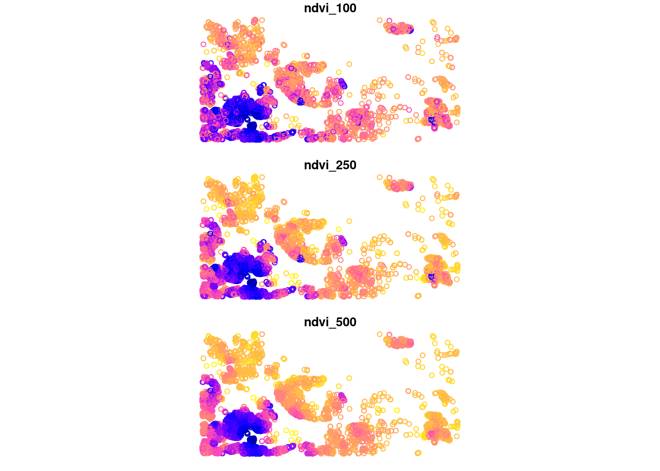
10    198.0

The median values extracted from the various buffers, for each point, are shown in Figure 5:

plot(pnt[c('ndvi_100', 'ndvi_250', 'ndvi_500')])