Linking exposures to residential adresses

Part 3: Distance to nearest polygon

Authors

Michael Dorman

Itai Kloog

Published

January 19, 2023

Download R script

Download data

1 Setup

library(sf)

Linking to GEOS 3.10.2, GDAL 3.4.1, PROJ 8.2.1; sf_use_s2() is TRUE

library(stars)

Loading required package: abind

2 Input data

2.1 Points

Importing the points:

pnt = st_read('data/export/Address coordinates.gpkg')

Reading layer `extracted' from data source 
  `/home/michael/Sync/presentations/p_2023_01_R_exposure_tutorial/data/export/Address coordinates.gpkg' 
  using driver `GPKG'
Simple feature collection with 13710 features and 2 fields
Geometry type: POINT
Dimension:     XY
Bounding box:  xmin: 669825 ymin: 6578850 xmax: 695023 ymax: 6590699
Projected CRS: SWEREF99 TM

pnt

Simple feature collection with 13710 features and 2 fields
Geometry type: POINT
Dimension:     XY
Bounding box:  xmin: 669825 ymin: 6578850 xmax: 695023 ymax: 6590699
Projected CRS: SWEREF99 TM
First 10 features:
   X_sw99_corr_final Y_sw99_corr_final                   geom
1            6579476            672969 POINT (672969 6579476)
2            6579535            672998 POINT (672998 6579535)
3            6580754            673589 POINT (673589 6580754)
4            6580685            670730 POINT (670730 6580685)
5            6580685            670730 POINT (670730 6580685)
6            6580707            670681 POINT (670681 6580707)
7            6580685            670730 POINT (670730 6580685)
8            6580063            671015 POINT (671015 6580063)
9            6581347            672437 POINT (672437 6581347)
10           6582407            673401 POINT (673401 6582407)

plot(st_geometry(pnt))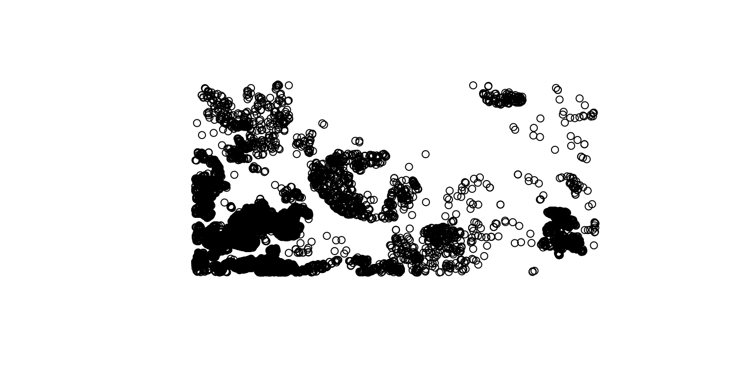

2.2 Polygons

Importing the polygons:

pol = st_read('data/export/water shapes/all Swedish water fixed.shp')

Reading layer `all Swedish water fixed' from data source 
  `/home/michael/Sync/presentations/p_2023_01_R_exposure_tutorial/data/export/water shapes/all Swedish water fixed.shp' 
  using driver `ESRI Shapefile'
Simple feature collection with 207 features and 7 fields
Geometry type: MULTIPOLYGON
Dimension:     XY
Bounding box:  xmin: 669800 ymin: 6578800 xmax: 695100 ymax: 6590700
Projected CRS: SWEREF99 TM

pol

Simple feature collection with 207 features and 7 fields
Geometry type: MULTIPOLYGON
Dimension:     XY
Bounding box:  xmin: 669800 ymin: 6578800 xmax: 695100 ymax: 6590700
Projected CRS: SWEREF99 TM
First 10 features:
    osm_id code fclass           name FID                     layer
1  4231060 8200  water    Brunnsviken  NA inner water OSM Swereff99
2  4875777 8200  water           <NA>  NA inner water OSM Swereff99
3  4875985 8200  water      Laduviken  NA inner water OSM Swereff99
4  4880167 8200  water           <NA>  NA inner water OSM Swereff99
5  4880274 8200  water           <NA>  NA inner water OSM Swereff99
6  4880745 8200  water  Kottlasj\xf6n  NA inner water OSM Swereff99
7  4985481 8200  water \xd6sbysj\xf6n  NA inner water OSM Swereff99
8  4985482 8200  water   Ekebysj\xf6n  NA inner water OSM Swereff99
9  5174088 8200  water           <NA>  NA inner water OSM Swereff99
10 5192316 8200  water           <NA>  NA inner water OSM Swereff99
                                                      path
1  C:/Users/anpyko/Downloads/inner water OSM Swereff99.shp
2  C:/Users/anpyko/Downloads/inner water OSM Swereff99.shp
3  C:/Users/anpyko/Downloads/inner water OSM Swereff99.shp
4  C:/Users/anpyko/Downloads/inner water OSM Swereff99.shp
5  C:/Users/anpyko/Downloads/inner water OSM Swereff99.shp
6  C:/Users/anpyko/Downloads/inner water OSM Swereff99.shp
7  C:/Users/anpyko/Downloads/inner water OSM Swereff99.shp
8  C:/Users/anpyko/Downloads/inner water OSM Swereff99.shp
9  C:/Users/anpyko/Downloads/inner water OSM Swereff99.shp
10 C:/Users/anpyko/Downloads/inner water OSM Swereff99.shp
                         geometry
1  MULTIPOLYGON (((671255.4 65...
2  MULTIPOLYGON (((680891 6585...
3  MULTIPOLYGON (((674562.9 65...
4  MULTIPOLYGON (((672992.5 65...
5  MULTIPOLYGON (((671457.4 65...
6  MULTIPOLYGON (((680554.1 65...
7  MULTIPOLYGON (((673763.5 65...
8  MULTIPOLYGON (((673078.9 65...
9  MULTIPOLYGON (((670779.9 65...
10 MULTIPOLYGON (((676609.2 65...

plot(st_geometry(pol), col = 'lightblue')
plot(st_geometry(pnt), add = TRUE)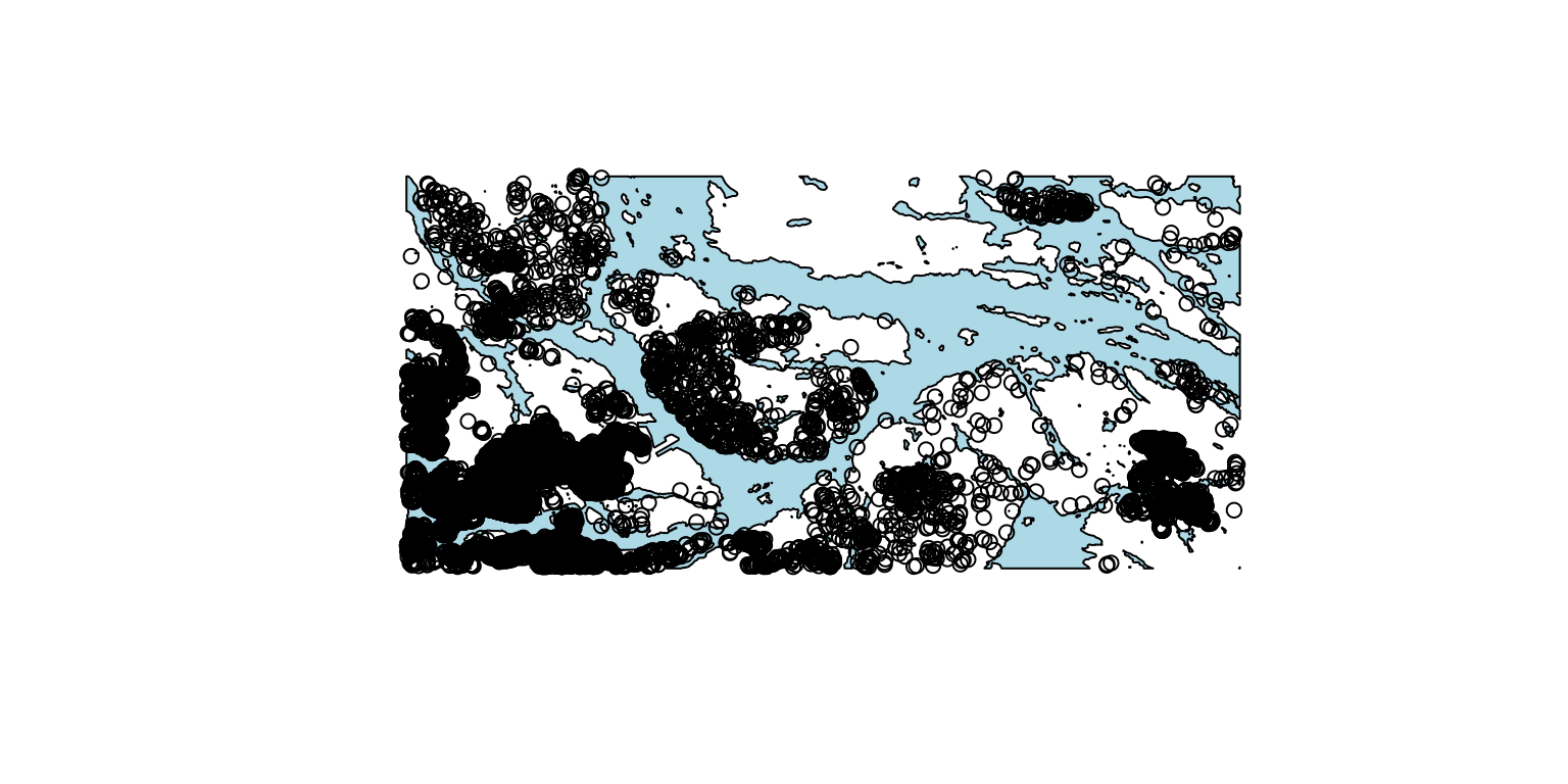

3 Distance to nearest polygon

To calculate the distance from each point to the nearest polygon, we use two sf functions:

st_union—to “dissolve” the polygon layer into one multipart geometry (since we are interested in the mininal distance to any polygon, not the specific distances to each polygon), and
st_distance—to calculate the distances,

as follows:

d = st_distance(pnt, st_union(pol))

The result d is a pairwise distance matrix, where rows correspond to pnt geometries and columns correspond to st_union(pol) geometries. In this case d has just one column, because st_union(pol) has just one geometry:

head(d)

Units: [m]
          [,1]
[1,] 192.70235
[2,] 145.22744
[3,]  39.13382
[4,] 169.15875
[5,] 169.15875
[6,] 166.07230

The distance values can be assigned to an attribute named "dist" in pnt, as follows:

pnt$dist = d[, 1]
pnt

Simple feature collection with 13710 features and 3 fields
Geometry type: POINT
Dimension:     XY
Bounding box:  xmin: 669825 ymin: 6578850 xmax: 695023 ymax: 6590699
Projected CRS: SWEREF99 TM
First 10 features:
   X_sw99_corr_final Y_sw99_corr_final                   geom          dist
1            6579476            672969 POINT (672969 6579476) 192.70235 [m]
2            6579535            672998 POINT (672998 6579535) 145.22744 [m]
3            6580754            673589 POINT (673589 6580754)  39.13382 [m]
4            6580685            670730 POINT (670730 6580685) 169.15875 [m]
5            6580685            670730 POINT (670730 6580685) 169.15875 [m]
6            6580707            670681 POINT (670681 6580707) 166.07230 [m]
7            6580685            670730 POINT (670730 6580685) 169.15875 [m]
8            6580063            671015 POINT (671015 6580063) 174.67891 [m]
9            6581347            672437 POINT (672437 6581347) 190.32676 [m]
10           6582407            673401 POINT (673401 6582407) 405.91121 [m]

Like in all distance- and area-related calculations in sf, the results are returned as units objects (R package units). This has some advantages, such as easier unit conversion, otherwise the behavior is similar to plain numeric values. In case we want to drop the units and get ordinary numeric values:

pnt$dist = as.numeric(pnt$dist)
pnt

Simple feature collection with 13710 features and 3 fields
Geometry type: POINT
Dimension:     XY
Bounding box:  xmin: 669825 ymin: 6578850 xmax: 695023 ymax: 6590699
Projected CRS: SWEREF99 TM
First 10 features:
   X_sw99_corr_final Y_sw99_corr_final                   geom      dist
1            6579476            672969 POINT (672969 6579476) 192.70235
2            6579535            672998 POINT (672998 6579535) 145.22744
3            6580754            673589 POINT (673589 6580754)  39.13382
4            6580685            670730 POINT (670730 6580685) 169.15875
5            6580685            670730 POINT (670730 6580685) 169.15875
6            6580707            670681 POINT (670681 6580707) 166.07230
7            6580685            670730 POINT (670730 6580685) 169.15875
8            6580063            671015 POINT (671015 6580063) 174.67891
9            6581347            672437 POINT (672437 6581347) 190.32676
10           6582407            673401 POINT (673401 6582407) 405.91121

plot(pnt['dist'], reset = FALSE)
plot(st_geometry(pol), col = '#0000ff20', add = TRUE)