Preface

Last updated: 2021-03-31 00:23:09

0.1 Welcome

This book contains the materials of the 3-credit undergraduate course named Introduction to Spatial Data Programming with R, given at the Department of Geography and Environmental Development, Ben-Gurion University of the Negev. The course was given in 2013, and then each year in the period 2015-2020. An earlier version of the materials was published by Packt (Dorman 2014)¹.

The structure of the book is as follows. This section (the Preface) introduces the R programming language, and shows some examples of its capabilities with respect to working with spatial data. In the main part of the book, the material is split in two parts:

Introduction to R programming (Chapters 1–4) gives all of the necessary knowledge on the R language required before we can start working with spatial data
Working with spatial data in R (Chapters 5–12) go over the main methods of working with spatial data in R, including how to process rasters, vector layers, and both, as well as two selected more advanced topics: spatio-temporal data and spatial interpolation

Finally, the appendices contain additional information:

Sample data used in the book (Appendix A)
Administrative details about the course (Appendix B)
Exercises (Appendices C–H)
Examples of exam questions (Appendix ??)

Hopefully, the text is detailed enough so that it can be used not only as course materials, but also for independent self-study.

0.2 What is R?

R is a programming language and environment, originally developed for statistical computing and graphics. As of October 2020, there are ~16,000 R packages in the official repository CRAN ².

Notable advantages of R are that it is a full-featured programming language, yet customized for working with data, relatively simple and has a huge collection of over 100,000 functions from various areas of interest.

R’s popularity has been steadily increasing in recent years (Figures 0.1–0.3).

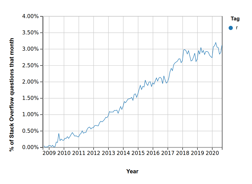
Figure 0.1: Stack Overflow Trend for the ‘r’ question tag (https://insights.stackoverflow.com/trends?tags=r)

Figure 0.2: IEEE Language Rankings 2019 (https://spectrum.ieee.org/computing/software/the-top-programming-languages-2019)

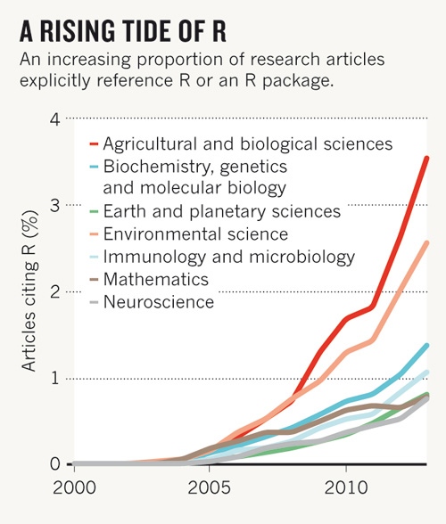
Figure 0.3: Proportion of research papers citing R (https://www.nature.com/news/programming-tools-adventures-with-r-1.16609)

A brief overview of the capabilities and packages for several domains of R use, are available in the “CRAN Task Views” (Figure 0.4).

Figure 0.4: CRAN Task Views (http://www.maths.lancs.ac.uk/~rowlings/R/TaskViews/)

0.3 R and analysis of spatial data

0.3.1 Introduction

Over time, there was an increasing number of contributed packages for handling and analyzing spatial data in R. Today, spatial analysis is a major functionality in R. As of October 2020, there are at least 185 packages³ specifically addressing spatial analysis in R.

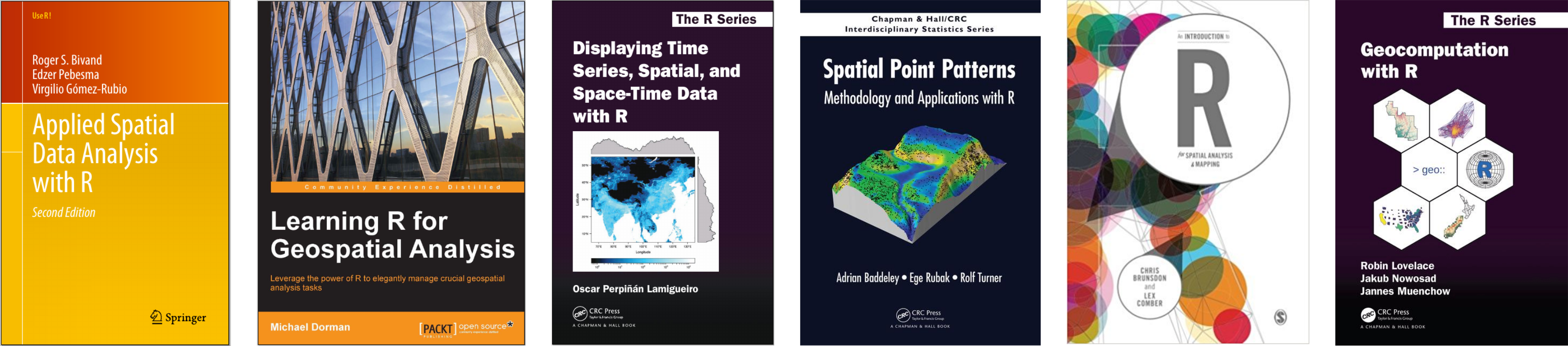
Figure 0.5: Books on Spatial Data Analysis with R

Some important events in the history of spatial analysis support in R are summarized in Table 0.1.

Table 0.1: Significant events in the history of R-spatial
Year	Event
pre-2003	Variable and incomplete approaches (`MASS`, `spatstat`, `maptools`, `geoR`, `splancs`, `gstat`, …)
2003	Consensus that a package defining standard data structures should be useful; `rgdal` released on CRAN
2005	`sp` released on CRAN; `sp` support in `rgdal` (Section 7.1.3
2008	Applied Spatial Data Analysis with R, 1^st ed.
2010	`raster` released on CRAN (Section 5.3.4)
2011	`rgeos` released on CRAN
2013	Applied Spatial Data Analysis with R, 2^nd ed.
2016	`sf` released on CRAN (Section 7.1.4)
2018	`stars` released on CRAN (Section 5.3.5)
2019	Geocomputation with R (https://geocompr.robinlovelace.net/)
2021(?)	Spatial Data Science (https://www.r-spatial.org/book/)

The question that arises here is: can R be used as a Geographic Information System (GIS), or as a comprehensive toolbox for doing spatial analysis? The answer is definitely yes. Moreover, R has some important advantages over traditional approaches to GIS, i.e., software with graphical user interfaces such as ArcGIS or QGIS.

General advantages of Command Line Interface (CLI) software include:

Automation—Doing otherwise unfeasible repetitive tasks
Reproducibility—Precise control of instructions to the computer

Moreover, specific strengths of R as a GIS are:

R capabilities in data processing and visualization, combined with dedicated packages for spatial data
A single environment encompassing all analysis aspects—acquiring data, computation, statistics, visualization, Web, etc.

Nevertheless, there are situations when other tools are needed:

Interactive editing or georeferencing (but see mapedit package)
Unique GIS algorithms (3D analysis, label placement, splitting lines at intersections)
Data that cannot fit in RAM (but R can connect to spatial databases⁴ and other softwere for working with big data)

The following sections (0.3.2–0.3.11) highlight some of the capabilities of spatial data analysis packages in R, through short examples. We are going to elaborate on most of these packages later on in the book, and many of those examples will become clear.

0.3.2 Input and output of spatial data

Reading spatial layers from a file into an R data structure, or writing the R data structure into a file, are handled by external libraries:

GDAL/OGR is used for reading/writing vector and raster files, with sf and stars
PROJ is used for handling Coordinate Reference Systems (CRS), in both sf and stars
Working with specialized formats, e.g., NetCDF with ncdf4

Package sf combined with RPostgreSQL can be used to read from, and write to, a PostGIS spatial database:

library(sf)
library(RPostgreSQL)
con = dbConnect(
  PostgreSQL(),
  dbname = "gisdb",
  host = "159.89.13.241",
  port = 5432,
  user = "geobgu",
  password = "*******"
)
dat = st_read(con, query = "SELECT name_lat, geometry FROM plants LIMIT 5;")

dat
## Simple feature collection with 5 features and 1 field
## Geometry type: POINT
## Dimension:     XY
## Bounding box:  xmin: 35.1397 ymin: 31.44711 xmax: 35.67976 ymax: 32.77013
## Geodetic CRS:  WGS 84
##         name_lat                  geometry
## 1    Iris haynei POINT (35.67976 32.77013)
## 2    Iris haynei   POINT (35.654 32.74137)
## 3 Iris atrofusca POINT (35.19337 31.44711)
## 4 Iris atrofusca POINT (35.18914 31.51475)
## 5  Iris vartanii  POINT (35.1397 31.47415)

0.3.3 `sf`: Processing Vector Layers

GEOS is used for geometric operations on vector layers with sf:

Numeric operators—Area, Length, Distance…
Logical operators—Contains, Within, Within distance, Crosses, Overlaps, Equals, Intersects, Disjoint, Touches…
Geometry generating operators—Centroid, Buffer, Intersection, Union, Difference, Convex-Hull, Simplification…

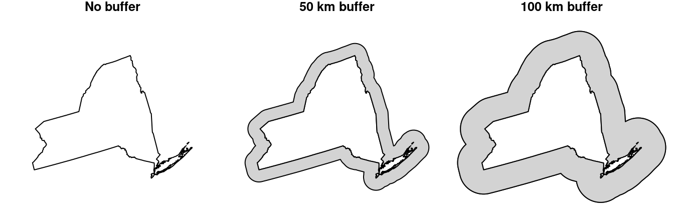
Figure 0.6: Buffer function

0.3.4 `stars`: Processing Rasters

Geometric operations on rasters can be done with package stars:

Accessing cell values—As matrix / array, Extracting to points / lines / polygons
Raster algebra—Arithmetic (+, -, …), Math (sqrt, log10, …), logical (!, ==, >, …), summary (mean, max, …), Masking
Changing resolution and extent—Cropping, Mosaic, Resampling, Reprojection
Transformations—Raster <-> Points / Contour lines / Polygons

0.3.5 `geosphere`: Geometric calculations on longitude/latitude

Package geosphere implements spherical geometry functions for distance- and direction-related calculations on geographic coordinates (lon-lat).

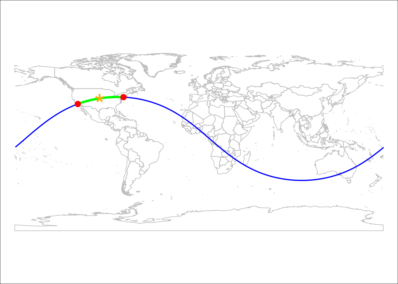
Figure 0.7: Points on Great Circle

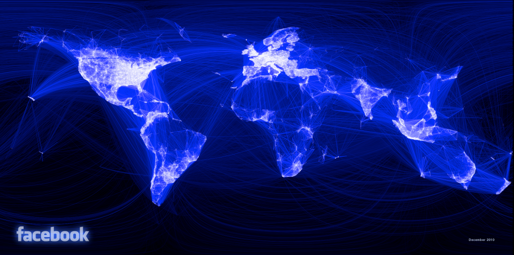
Figure 0.8: Visualizing Facebook Friends with geosphere (http://paulbutler.org/archives/visualizing-facebook-friends/)

0.3.6 `gstat`: Geostatistical Modelling

As mentioned above, R was initially developed for statistical computing (Section 0.2). Accordingly, there is an extensive set of R packages for spatial statistics. For example, package gstat provides a comprehensive set of functions for univariate and multivariate geostatistics, mainly for the purpose of spatial interpolation:

Variogram modelling
Ordinary and universal point or block (co)kriging
Cross-validation

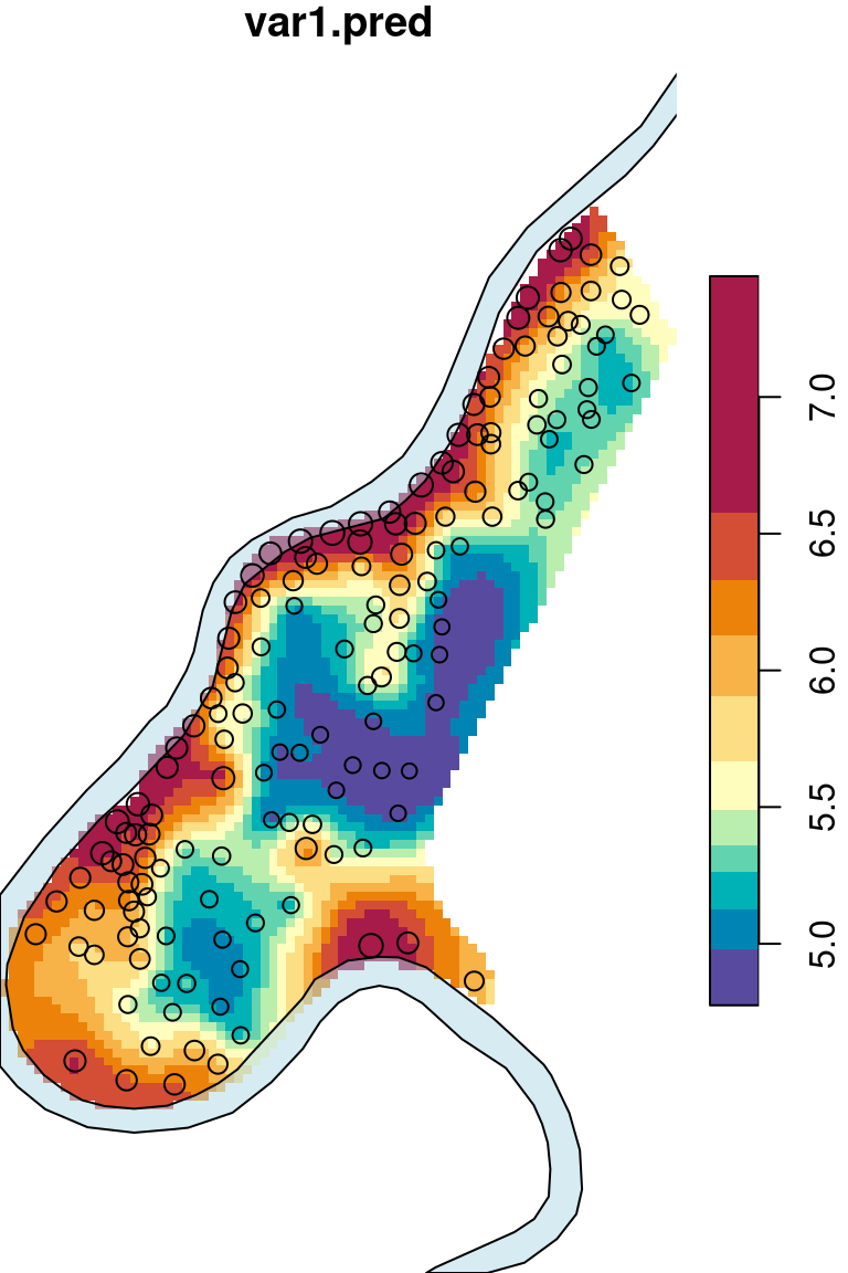
Figure 0.9: Predicted Zinc concentration, using Ordinary Kriging

We are going to learn about the gstat package in Chapter 12. An introduction to the package can also be found in Chapter 8 of Applied Spatial Data Analysis with R (Bivand, Pebesma, and Gomez-Rubio 2013).

0.3.7 `spdep`: Spatial dependence modelling

Modelling with spatial weights:

Building neighbor lists and spatial weights
Tests for spatial autocorrelation for areal data (e.g., Moran’s I)
Spatial regression models (e.g., SAR, CAR)

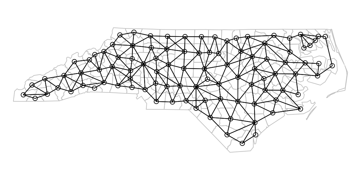
Figure 0.10: Neighbours list based on regions with contiguous boundaries

The spdep package is beyond the scope of this book. An introduction to the package can be found in Chapter 9 of Applied Spatial Data Analysis with R (Bivand, Pebesma, and Gomez-Rubio 2013).

0.3.8 `spatstat`: Spatial point pattern analysis

Package spatstat provides a comprehensive collection of techniques for statistical analysis of spatial point patterns, such as:

Kernel density estimation
Detection of clustering using Ripley’s K-function
Spatial logistic regression

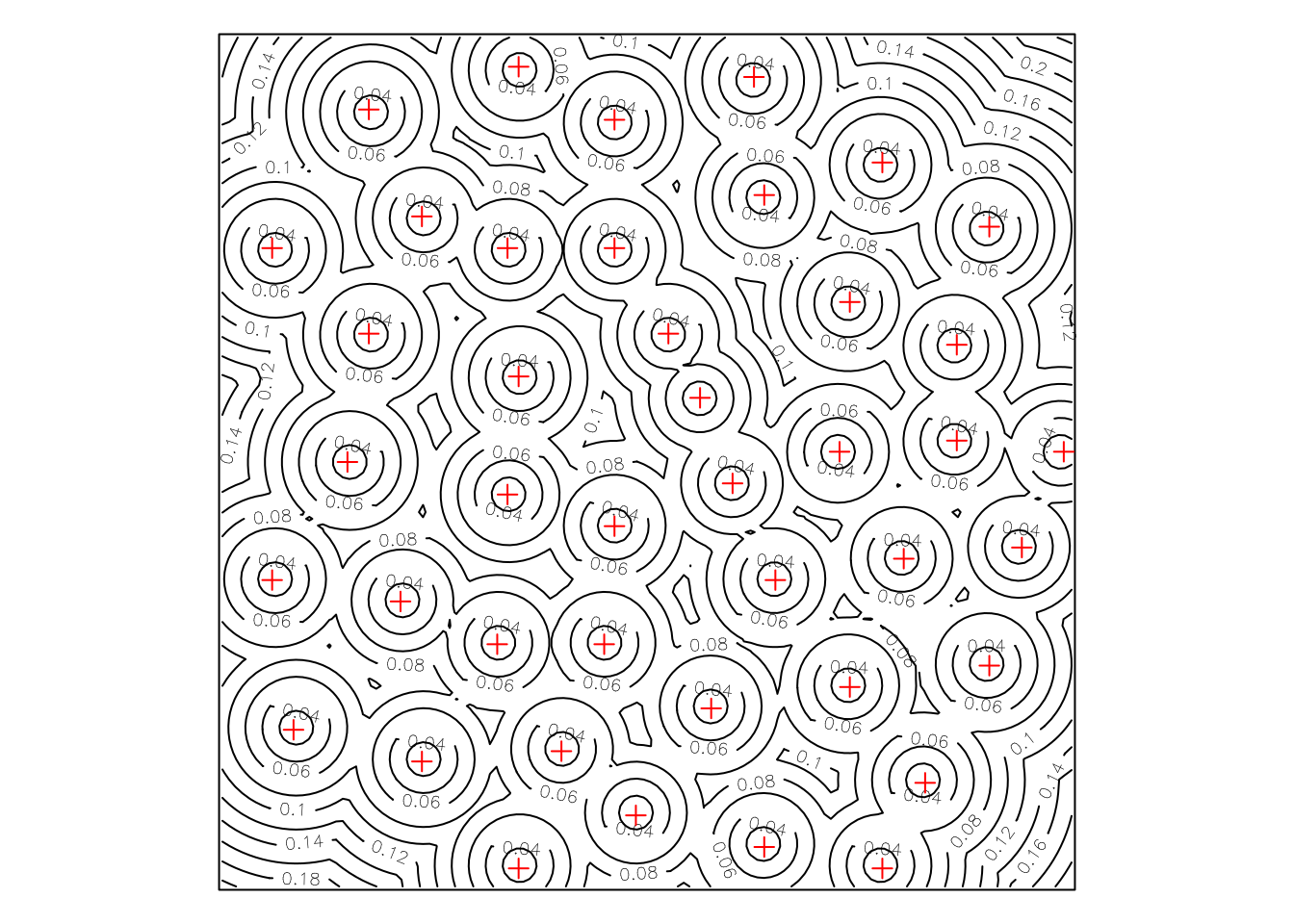
Figure 0.11: Distance map for the Biological Cells point pattern dataset

The book Spatial point patterns: methodology and applications with R (Baddeley, Rubak, and Turner 2015) provides a thorough introduction to the subject of point pattern analysis using the spatstat package. A more brief introduction can also be found in Chapter 7 of Applied Spatial Data Analysis with R (Bivand, Pebesma, and Gomez-Rubio 2013).

0.3.9 `osmdata`: Access to OpenStreetMap data

Package osmdata gives access to OpenStreetMap (OSM) data—the most extensive open-source map database in the worls—using the Overpass API⁵.

library(sf)
library(osmdata)
q = opq(bbox = "Beer-Sheva, Israel")
q = add_osm_feature(q, key = "highway")
dat = osmdata_sf(q)
lines = dat$osm_lines
pol = dat$osm_polygons
pol = st_cast(pol, "MULTILINESTRING")
pol = st_cast(pol, "LINESTRING")
lines = rbind(lines, pol)
lines = lines[, "highway"]
lines = st_transform(lines, 32636)
plot(lines, key.pos = 4, key.width = lcm(4), main = "")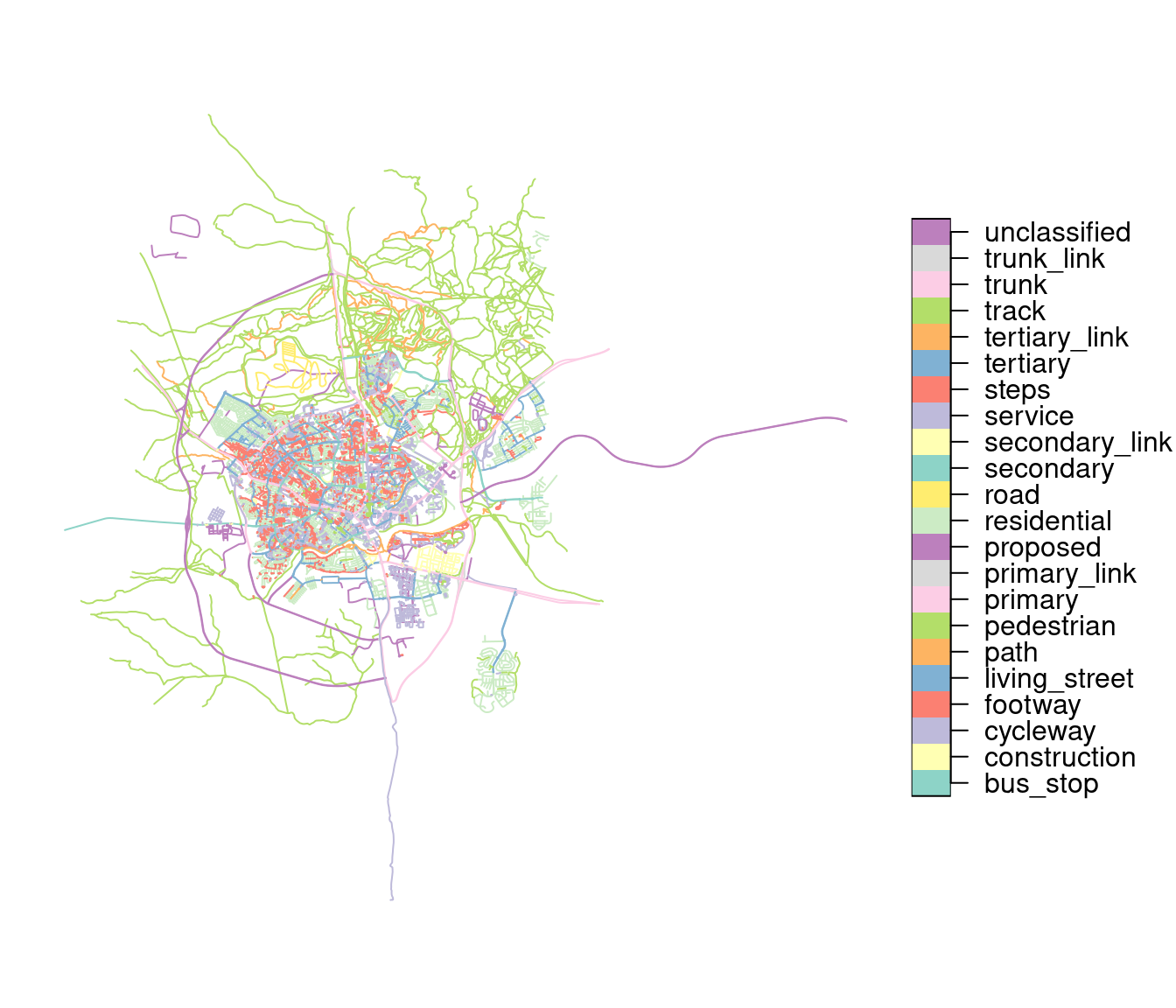

Figure 0.12: Beer-Sheva road types map, using data downloaded from OpenStreetMap (OSM)

0.3.10 `ggplot2`: Visualization

The ggplot2 package is one of the most popular packages in R. It provides advanced visualization methods through a well-designed and consistent syntax. The package supports visualization of both vector layers⁶ and rasters⁷.

The ggplot2 package is highly customizable and capable of producing publication-quality figures and maps as well as original and innovative designs (Figure 0.13). One of its strengths is in easy preparation of “small-multiple”—or facet, in the terminology of ggplot2—figures (Figure 0.14).

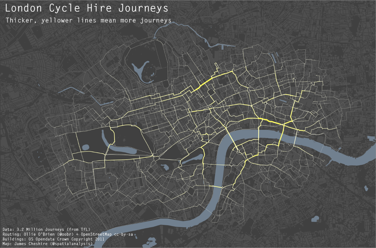
Figure 0.13: London cycle hire journeys with ggplot2 (http://spatial.ly/2012/02/great-maps-ggplot2/)

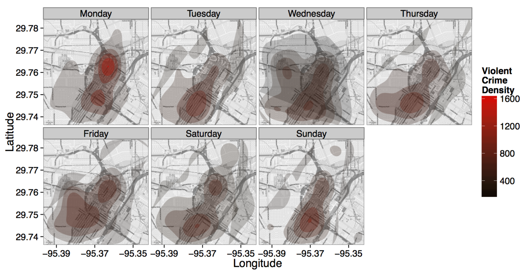
Figure 0.14: Crime density by day with ggplot2

The ggplot2 package is beyond the scope of this book. A good place to start is the book ggplot2: Elegant Graphics for Data Analysis, by package author (Wickham 2016). The book is available online⁸.

0.3.11 `leaflet`, `mapview`: Web mapping

Packages leaflet and mapview provide methods to produce interactive maps using the Leaflet JavaScript library.

Package leaflet gives more low-level control. Package mapview is a wrapper around leaflet, automating addition of useful features:

Commonly used basemaps
Color scales and legends
Labels
Popups

Function mapview produces an interactive map given a spatial object. The zcol parameter is used to specify the attribute used for symbology:

library(sf)
library(mapview)
states = st_read("USA_2_GADM_fips.shp")
mapview(states, zcol = "NAME_1")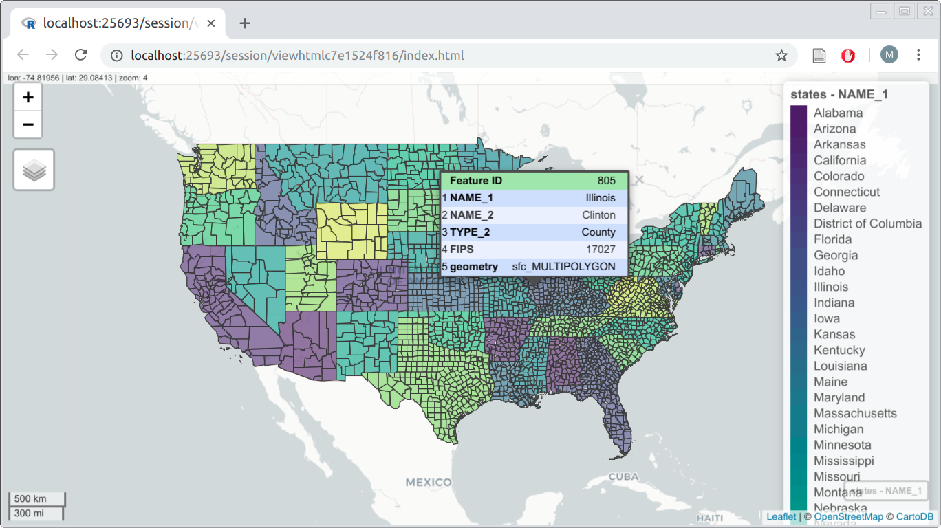

Figure 0.15: Intractive map made with mapview

0.4 Other materials

This section lists some other resources that are relevant for working with spatial data in R.

0.4.1 Books

Model-based Geostatistics (Diggle and Ribeiro 2007)
A Practical Guide to Geostatistical Mapping (Hengl 2009)
Spatial Data Analysis in Ecology and Agriculture using R (1^st ed. 2012, 2^nd ed. 2018) (Plant 2018)
Learning R for Geospatial Analysis (Dorman 2014)
Applied Spatial Data Analysis with R (1^st ed. 2008, 2^nd ed. 2013) (Bivand, Pebesma, and Gomez-Rubio 2013)
Hierarchical Modeling and Analysis for Spatial Data (1^st ed. 2003, 2^nd ed. 2014) (Banerjee, Carlin, and Gelfand 2014)
An Introduction to R for Spatial Analysis and Mapping (1^st ed. 2015, 2^nd ed. 2018) (Brunsdon and Comber 2015)
Spatial Point Patterns: Methodology and Applications with R (2015) (Baddeley, Rubak, and Turner 2015)
Displaying Time Series, Spatial, and Space-Time Data with R (1^st ed. 2014, 2^nd ed. 2018) (Lamigueiro 2014)
Predictive Soil Mapping with R (Hengl and MacMillan 2019)
Geocomputation with R (Lovelace, Nowosad, and Muenchow 2019)
Spatial Data Science (2021?)

0.4.2 Papers

Pebesma, E., Bivand, R. S. (2005). Classes and Methods for Spatial Data: the sp Package. R news, 5(2), 9-13. [PDF]
Pebesma, E. (2018). Simple Features for R: Standardized Support for Spatial Vector Data. The R Journal, 10(1):439-446. [PDF]

Introduction to Spatial Data Programming with R

Introduction to Spatial Data Programming with R

Preface

0.1 Welcome

0.2 What is R?

0.3 R and analysis of spatial data

0.3.1 Introduction

0.3.2 Input and output of spatial data

0.3.3 `sf`: Processing Vector Layers

0.3.4 `stars`: Processing Rasters

0.3.5 `geosphere`: Geometric calculations on longitude/latitude

0.3.6 `gstat`: Geostatistical Modelling

0.3.7 `spdep`: Spatial dependence modelling

0.3.8 `spatstat`: Spatial point pattern analysis

0.3.9 `osmdata`: Access to OpenStreetMap data

0.3.10 `ggplot2`: Visualization

0.3.11 `leaflet`, `mapview`: Web mapping

0.4 Other materials

0.4.1 Books

0.4.2 Papers

0.4.3 Courses and tutorials

0.4.3.1 Courses

0.4.3.2 Tutorials

0.4.3.3 Presentations

0.4.3.4 Official materials

Introduction to Spatial Data Programming with R

Preface

0.1 Welcome

0.2 What is R?

0.3 R and analysis of spatial data

0.3.1 Introduction

0.3.2 Input and output of spatial data

0.3.3 sf: Processing Vector Layers

0.3.4 stars: Processing Rasters

0.3.5 geosphere: Geometric calculations on longitude/latitude

0.3.6 gstat: Geostatistical Modelling

0.3.7 spdep: Spatial dependence modelling

0.3.8 spatstat: Spatial point pattern analysis

0.3.9 osmdata: Access to OpenStreetMap data

0.3.10 ggplot2: Visualization

0.3.11 leaflet, mapview: Web mapping

0.4 Other materials

0.4.1 Books

0.4.2 Papers

0.4.3 Courses and tutorials

0.4.3.1 Courses

0.4.3.2 Tutorials

0.4.3.3 Presentations

0.4.3.4 Official materials

0.3.3 `sf`: Processing Vector Layers

0.3.4 `stars`: Processing Rasters

0.3.5 `geosphere`: Geometric calculations on longitude/latitude

0.3.6 `gstat`: Geostatistical Modelling

0.3.7 `spdep`: Spatial dependence modelling

0.3.8 `spatstat`: Spatial point pattern analysis

0.3.9 `osmdata`: Access to OpenStreetMap data

0.3.10 `ggplot2`: Visualization

0.3.11 `leaflet`, `mapview`: Web mapping