Linking exposures to residential adresses

Part 4: Extracting from mesh

Authors

Michael Dorman

Itai Kloog

Published

January 19, 2023

Download R script

Download data

1 Setup

library(sf)

Linking to GEOS 3.10.2, GDAL 3.4.1, PROJ 8.2.1; sf_use_s2() is TRUE

library(stars)

Loading required package: abind

2 Input data

2.1 Points

Importing the points:

pnt = st_read('data/export/Address coordinates.gpkg')

Reading layer `extracted' from data source 
  `/home/michael/Sync/presentations/p_2023_01_R_exposure_tutorial/data/export/Address coordinates.gpkg' 
  using driver `GPKG'
Simple feature collection with 13710 features and 2 fields
Geometry type: POINT
Dimension:     XY
Bounding box:  xmin: 669825 ymin: 6578850 xmax: 695023 ymax: 6590699
Projected CRS: SWEREF99 TM

pnt

Simple feature collection with 13710 features and 2 fields
Geometry type: POINT
Dimension:     XY
Bounding box:  xmin: 669825 ymin: 6578850 xmax: 695023 ymax: 6590699
Projected CRS: SWEREF99 TM
First 10 features:
   X_sw99_corr_final Y_sw99_corr_final                   geom
1            6579476            672969 POINT (672969 6579476)
2            6579535            672998 POINT (672998 6579535)
3            6580754            673589 POINT (673589 6580754)
4            6580685            670730 POINT (670730 6580685)
5            6580685            670730 POINT (670730 6580685)
6            6580707            670681 POINT (670681 6580707)
7            6580685            670730 POINT (670730 6580685)
8            6580063            671015 POINT (671015 6580063)
9            6581347            672437 POINT (672437 6581347)
10           6582407            673401 POINT (673401 6582407)

plot(st_geometry(pnt))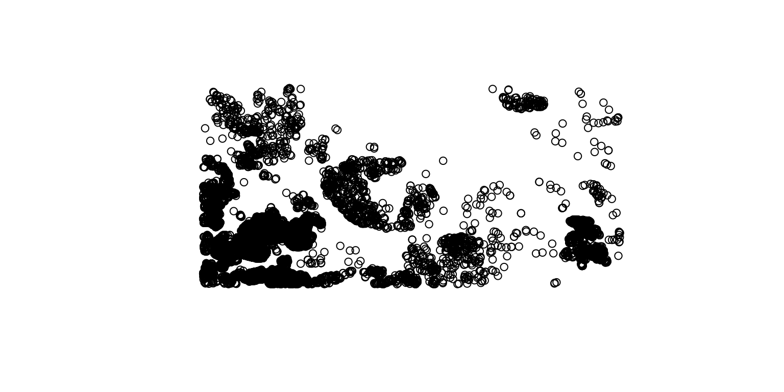

2.2 Mesh

Conversion from mesh (.2dm) to GeoTIFF (.tif) can be done using the QGIS tool named native:meshrasterize, from within R:

x = 'qgis_process run native:meshrasterize -- INPUT="data/export/Noise/Road traffic/Road_traffic_noise_2018_L_PF.2dm" DATASET_GROUPS="0" DATASET_TIME="2022-01-15" PIXEL_SIZE="20" OUTPUT="tmp.tif"'
system(x)

or from the command line:

export QT_QPA_PLATFORM="offscreen"
qgis_process run native:meshrasterize -- INPUT="data/export/Noise/Road traffic/Road_traffic_noise_2018_L_PF.2dm" DATASET_GROUPS="0" DATASET_TIME="2022-01-15" PIXEL_SIZE="20" OUTPUT="tmp.tif"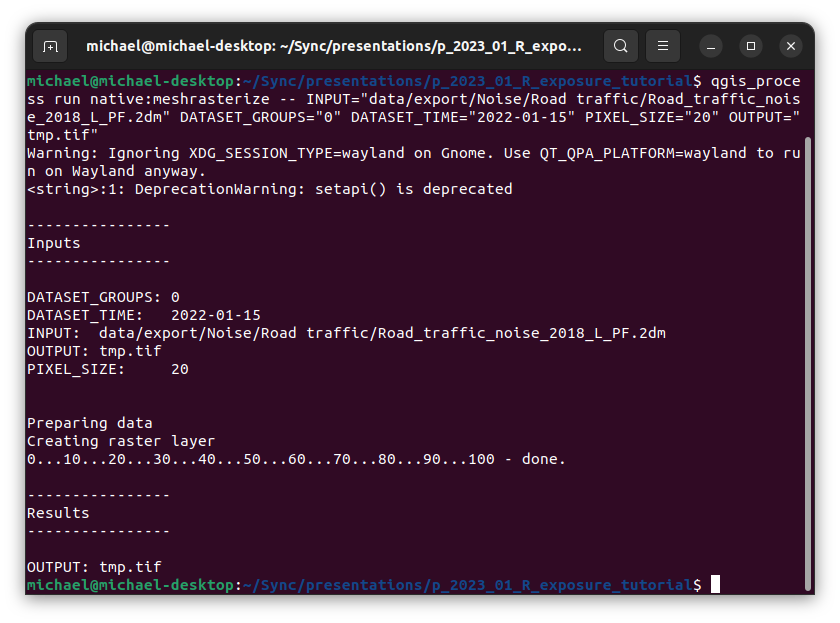

The raster file we got from qgis_process can be imported back into the R environment:

r = read_stars('tmp.tif')
names(r) = 'traffic_noise'
r

stars object with 2 dimensions and 1 attribute
attribute(s):
                 Min. 1st Qu. Median     Mean 3rd Qu. Max.
traffic_noise  15.097  26.694 40.307 39.88116  52.746   75
dimension(s):
  from   to  offset    delta refsys point values x/y
x    1 1262  669825  20.0079     NA    NA   NULL [x]
y    1  592 6590700 -20.0169     NA    NA   NULL [y]

In this case the CRS definition is missing:

st_crs(r)

Coordinate Reference System: NA

We can set it as follows, based on prior knowledge that the raster CRS is the same as the points layer CRS:

st_crs(r) = st_crs(pnt)
r

stars object with 2 dimensions and 1 attribute
attribute(s):
                 Min. 1st Qu. Median     Mean 3rd Qu. Max.
traffic_noise  15.097  26.694 40.307 39.88116  52.746   75
dimension(s):
  from   to  offset    delta      refsys point values x/y
x    1 1262  669825  20.0079 SWEREF99 TM    NA   NULL [x]
y    1  592 6590700 -20.0169 SWEREF99 TM    NA   NULL [y]

plot(r, col = hcl.colors(11, 'Spectral', rev = TRUE), reset = FALSE)
plot(st_geometry(pnt), add = TRUE)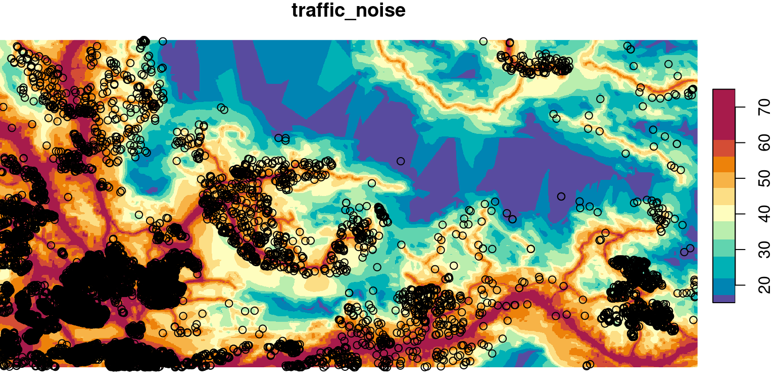

3 Extracting raster values to points

Now the raster values can be extracted to points using st_extract as shown previously (see Part 1):

pnt$traffic_noise = st_extract(r, pnt)[[1]]
pnt

Simple feature collection with 13710 features and 3 fields
Geometry type: POINT
Dimension:     XY
Bounding box:  xmin: 669825 ymin: 6578850 xmax: 695023 ymax: 6590699
Projected CRS: SWEREF99 TM
First 10 features:
   X_sw99_corr_final Y_sw99_corr_final                   geom traffic_noise
1            6579476            672969 POINT (672969 6579476)        57.981
2            6579535            672998 POINT (672998 6579535)        55.749
3            6580754            673589 POINT (673589 6580754)        61.455
4            6580685            670730 POINT (670730 6580685)        63.560
5            6580685            670730 POINT (670730 6580685)        63.560
6            6580707            670681 POINT (670681 6580707)        64.200
7            6580685            670730 POINT (670730 6580685)        63.560
8            6580063            671015 POINT (671015 6580063)        64.197
9            6581347            672437 POINT (672437 6581347)        63.831
10           6582407            673401 POINT (673401 6582407)        57.880

plot(pnt['traffic_noise'])