3 Rasters

3.1 Loading packages

import matplotlib.pyplot as plt
import geopandas as gpd
import rasterio
import rasterio.plot

3.2 Reading from file

The rasterio package works with the concept of a file connection. A raster file connection has two components:

The metadata (such as the dimensions, resolution, CRS, etc.)
A reference to the raster values (Figure 3.1)

When necessary, the values can be read into memory, either all at once, or from a particular band and/or “window”, or at a particular resolution. The rationale is that the metadata are small (and often useful to examine on their own), while values are often very big. Therefore, it can be more practical to have control over which values to read, and when.

Figure 3.1: Raster (`rasterio`) structure

To create a file connection object to a raster file, we use the rasterio.open function. For example, here we create a file connection object named src, which refers to the HEF_res200-M.tif raster. This is an aerial photograph of the Haifa area, downloaded from data.gov.il:

src = rasterio.open('data/HEF_res200-M.tif')
src

<open DatasetReader name='data/HEF_res200-M.tif' mode='r'>

The raster metadata can be accessed through the .src property of the file connection. For example, from the following metadata object:

src.meta

{'driver': 'GTiff',
 'dtype': 'uint8',
 'nodata': None,
 'width': 10000,
 'height': 10000,
 'count': 4,
 'crs': CRS.from_epsg(2039),
 'transform': Affine(2.0, 0.0, 190000.0,
        0.0, -2.0, 760000.0)}

we can learn that:

Raster data type is unsigned 8-bit integers (uint8), i.e., 0-255
Raster size is \(10,000\times10,000\) pixels
Raster has 4 bands (bands 1-3 are RGB, unclear what the 4^th band is…)
Raster CRS is ITM (EPSG:2039)
Raster resolution is 2 \(m\)

The raster values can be read using the .read method. The default is to read all values (as mentioned above, there are many other options to read partial data):

r = src.read()
r

array([[[255, 255, 255, ..., 130, 113,  81],
        [255, 255, 255, ..., 137, 130,  86],
        [255, 255, 255, ...,  45, 120, 121],
        ...,
        [255, 255, 255, ..., 207, 116,  53],
        [255, 255, 255, ..., 129, 192, 185],
        [255, 255, 255, ..., 179,  61,  68]],

       [[255, 255, 255, ..., 128, 109,  83],
        [255, 255, 255, ..., 133, 128,  79],
        [255, 255, 255, ...,  42, 119, 121],
        ...,
        [255, 255, 255, ..., 217, 103,  63],
        [255, 255, 255, ..., 128, 193, 184],
        [255, 255, 255, ..., 179,  61,  69]],

       [[255, 255, 255, ..., 122, 109,  78],
        [255, 255, 255, ..., 128, 124,  77],
        [255, 255, 255, ...,  46, 116, 115],
        ...,
        [255, 255, 255, ..., 218, 117,  78],
        [255, 255, 255, ..., 125, 189, 176],
        [255, 255, 255, ..., 174,  67,  74]],

       [[255, 255, 255, ..., 255, 255, 255],
        [255, 255, 255, ..., 255, 255, 255],
        [255, 255, 255, ..., 255, 255, 255],
        ...,
        [255, 255, 255, ..., 255, 255, 255],
        [255, 255, 255, ..., 255, 255, 255],
        [255, 255, 255, ..., 255, 255, 255]]], dtype=uint8)

The resulting object r is an ndarray object (package numpy):

type(r)

numpy.ndarray

The array stores the values using the same data type and the same precision as in the original file:

r.dtype

dtype('uint8')

This means that the minimal amount of RAM is being used, which is an advantage of Python over other programming languages such as R.

3.3 Plotting

The show function (from the rasterio.plot “sub-package”) can be used to plot a raster. This function can accept, and read from, a file connection. The rasterio.plot.show function automatically assumes that the first three bands refer to RGB with range 0-255, which is very common and exactly our case (otherwise we can rescale the values and/or rearrange the bands).

For example:

rasterio.plot.show(src);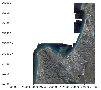

Here is an example of displaying both a raster and a vector layer in the same plot. The technique is the same as when displaying two or more vector layers (see Section 2.4):

pol = gpd.read_file('data/TAZ_NORTH_POPDENS_2016.shp')
fig, ax = plt.subplots()
rasterio.plot.show(src, ax=ax)
pol.plot(ax=ax, edgecolor='black', linewidth=0.3, color='none');

3.4 Geoprocessing

As an example of raster processing, let’s apply a raster algebra operation to our raster. In the next example, we calculate a grayscale image. Given \(Red\), \(Green\), and \(Blue\), bands, a simple formula for a greyscale image is calculating the weighted average reflectance from all three bands, as follows:

\[Grey=0.2125 \times Red + 0.7154 \times Green + 0.0721 \times Blue\]

Here is how we can calculate a greyscale image from our aerial photograph, a using numpy vectorized arithmetic operation, where:

r[0] is the \(Red\) band,
r[1] is the \(Green\) band, and
r[2] is the \(Blue\) band.

The result greyscale is a single-band array with greyscale values:

greyscale = 0.2125*r[0] + 0.7154*r[1] + 0.0721*r[2]
greyscale

array([[255.    , 255.    , 255.    , ..., 127.9924, 109.85  ,  82.2145],
       [255.    , 255.    , 255.    , ..., 133.4895, 128.1366,  80.3433],
       [255.    , 255.    , 255.    , ...,  42.9259, 118.9962, 120.5674],
       ...,
       [255.    , 255.    , 255.    , ..., 214.9471, 106.7719,  61.9565],
       [255.    , 255.    , 255.    , ..., 127.9962, 192.4991, 183.6357],
       [255.    , 255.    , 255.    , ..., 178.6395,  61.4326,  69.148 ]])

A standalone numpy array, such as greyscale, can also be passed to rasterio.plot.show. If we want to display CRS coordinates, or other layers, we also need to pass the georeferencing information stored in the “transformation matrix”, such as src.transform:

rasterio.plot.show(greyscale, transform=src.transform, cmap='Greys_r');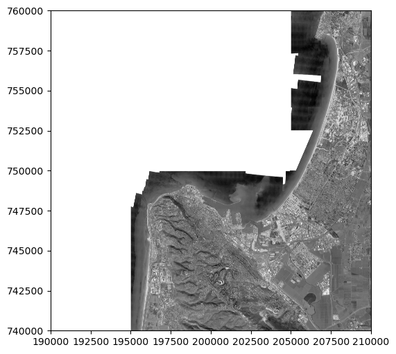

3.5 More information

See the Python Quickstart tutorial (Figure 3.2), and other sections in the rasterio documentation, for more information about rasterio.

Figure 3.2: The Python Quickstart tutorial