2  Vector layers

2.1 Loading packages

First, we import the two packages we will be working with:

• pandas—for working with tables, and
• geopandas—For working with vector layers,

as follows:

import pandas as pd
import geopandas as gpd

2.2 Table to point layer

In the first example, we are going to read an Excel file with x/y coordinates, and convert it to a (point) vector layer. The file bycode2019-2.xlsx contains town locations in Israel in 2019, downloaded from data.gov.il.

To read an Excel (.xlsx) file, we use the pd.read_excel function. The result is a data structure called DataFrame, used to represent a table in the pandas package:

dat = pd.read_excel('data/bycode2019-2.xlsx')
dat

	שם יישוב	סמל יישוב	תעתיק	...	שנה	שם יישוב באנגלית	אשכול רשויות מקומיות
0	אבו ג'ווייעד (שבט)	967	ABU JUWEI'ID	...	2019	Abu Juway'ad	NaN
1	אבו גוש	472	ABU GHOSH	...	2019	Abu Ghosh	NaN
2	אבו סנאן	473	ABU SINAN	...	2019	Abu Sinan	NaN
...	...	...	...	...	...	...	...
1480	תראבין א-צאנע (שבט)	970	TARABIN AS-SANI	...	2019	Tarabin as-Sani'	NaN
1481	תרבין א-צאנע (יישוב)*	1346	TARABIN AS-SANI	...	2019	Tarabin As-Sani	610.0
1482	תרום	778	TARUM	...	2019	Tarum	NaN

1483 rows × 23 columns

The column named “coordinates” contains the town coordinates:

dat['קואורדינטות']

0       2.040057e+09
1       2.105263e+09
2       2.160776e+09
            ...     
1480    1.830056e+09
1481    1.752658e+09
1482    1.983663e+09
Name: קואורדינטות, Length: 1483, dtype: float64

The following code section:

• filters out the rows with missing coordinate values, since these cannot be tranalated to point geometries, and
• splits the coordinate string to X and Y values, according to the instructions.

dat = dat[dat['קואורדינטות'].notna()].copy().reset_index(drop=True)
dat['x'] = dat['קואורדינטות'].astype(str).str.slice(0,5).astype(float) * 10
dat['y'] = dat['קואורדינטות'].astype(str).str.slice(5,10).astype(float) * 10

As a result, we now have x and y numeric columns with the ITM coordinates of each town:

dat

	שם יישוב	סמל יישוב	תעתיק	...	אשכול רשויות מקומיות	x	y
0	אבו ג'ווייעד (שבט)	967	ABU JUWEI'ID	...	NaN	204000.0	571000.0
1	אבו גוש	472	ABU GHOSH	...	NaN	210520.0	634810.0
2	אבו סנאן	473	ABU SINAN	...	NaN	216070.0	762840.0
...	...	...	...	...	...	...	...
1448	תראבין א-צאנע (שבט)	970	TARABIN AS-SANI	...	NaN	183000.0	564000.0
1449	תרבין א-צאנע (יישוב)*	1346	TARABIN AS-SANI	...	610.0	175260.0	583690.0
1450	תרום	778	TARUM	...	NaN	198360.0	632270.0

1451 rows × 25 columns

The two columns, along with the CRS definition (EPSG:2039 for ITM) can be transformed to a GeoSeries object. A GeoSeries is a sequence of geometries, along with the CRS definition, also known as the “geometry column” when it is part of a vector layer:

geom = gpd.points_from_xy(dat['x'], dat['y'], crs=2039)
geom = gpd.GeoSeries(geom)
geom

0       POINT (204000.000 571000.000)
1       POINT (210520.000 634810.000)
2       POINT (216070.000 762840.000)
                    ...              
1448    POINT (183000.000 564000.000)
1449    POINT (175260.000 583690.000)
1450    POINT (198360.000 632270.000)
Length: 1451, dtype: geometry

One of the first things we might want to do with a GeoSeries is to .plot it, to examine what it looks like:

geom.plot();

Combining a GeoSeries with a corresponding table yields GeoDataFrame object, a data structure representing a vector layer, where:

• The GeoSeries is the geometric/spatial part
• The DataFrame is the non-spatial/attributes part

For example, here we combine the GeoSeries named geom, with a DataFrame named dat, resulting in a GeoDataFrame named pnt:

pnt = gpd.GeoDataFrame(data=dat, geometry=geom)
pnt

	שם יישוב	סמל יישוב	תעתיק	...	x	y	geometry
0	אבו ג'ווייעד (שבט)	967	ABU JUWEI'ID	...	204000.0	571000.0	POINT (204000.000 571000.000)
1	אבו גוש	472	ABU GHOSH	...	210520.0	634810.0	POINT (210520.000 634810.000)
2	אבו סנאן	473	ABU SINAN	...	216070.0	762840.0	POINT (216070.000 762840.000)
...	...	...	...	...	...	...	...
1448	תראבין א-צאנע (שבט)	970	TARABIN AS-SANI	...	183000.0	564000.0	POINT (183000.000 564000.000)
1449	תרבין א-צאנע (יישוב)*	1346	TARABIN AS-SANI	...	175260.0	583690.0	POINT (175260.000 583690.000)
1450	תרום	778	TARUM	...	198360.0	632270.0	POINT (198360.000 632270.000)

1451 rows × 26 columns

Figure 2.1 summarizes the workflow of constructing a vector layer:

• Individual geometries—shapely objects (package shapely)
• Geometry column—GeoSeries objects
• Vector layer—GeoDataFrame object

Figure 2.1: Creating a GeoDataFrame from scratch

Figure 2.2 shows the hierarchical structure of GeoDataFrame, using another hypothetical vector layer with two points (London and Paris):

• The entire vector layer is a GeoDataFrame object
• The geometric part, i.e., the geometry column, is a GeoSeries object
• Each cell in the geometry column, i.e., an individual geometry, is a shapely object (package shapely)

Figure 2.2: Structure of a GeoDataFrame

2.3 Reading from file

Another common workflow with vector layers is to import an existing one, from a file. In the next example, we import a Shapefile named TAZ_NORTH_POPDENS_2016.shp. This is a polygonal layer with population density (POP_DENSE) extimates for Northern Israel. The Shapefile was downloaded from data.gov.il.

To import a vector layer from a file, we use the gpd.read_file function:

pol = gpd.read_file('data/TAZ_NORTH_POPDENS_2016.shp')
pol

	OBJECTID	POP_DENSE	SHAPE_Leng	...	POP2016	TAZ_AREA	geometry
0	1	1425.666870	13215.852473	...	9852	6.910450e+06	POLYGON ((217434.341 73558...
1	2	154.888062	21350.948435	...	2748	1.774185e+07	POLYGON ((215109.748 73483...
2	3	115.392609	20113.127398	...	2064	1.788676e+07	POLYGON ((212411.866 74531...
...	...	...	...	...	...	...	...
778	779	10459.399414	4026.527360	...	6828	6.528099e+05	POLYGON ((227634.472 72406...
779	780	1758.489014	3316.818207	...	1017	5.783374e+05	POLYGON ((226951.788 72387...
780	781	518.559326	20705.740930	...	5568	1.073744e+07	POLYGON ((226132.518 72486...

781 rows × 7 columns

We can see that the geometry type, in this case, is POLYGON.

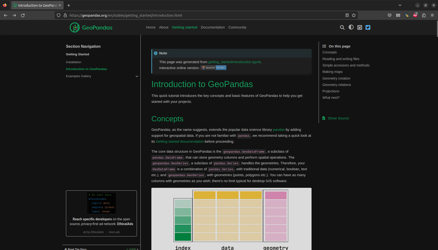
2.4 Plotting

By default, plotting a GeoDataFrame using .plot shows an image of the geometric part:

pol.plot();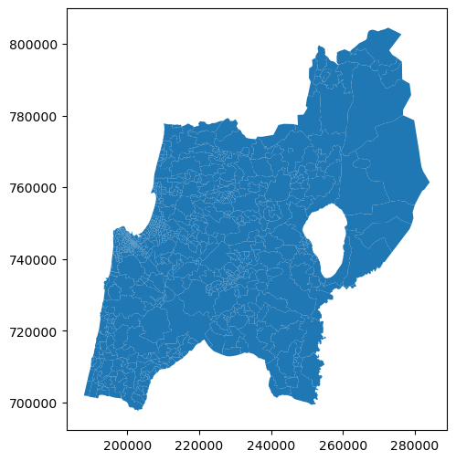

We can add symbology and legend, according to an attribute, using the column and legend=True arguments. For example, here we display the population density estimates (POP_DENSE attributes):

pol.plot(column='POP_DENSE', legend=True);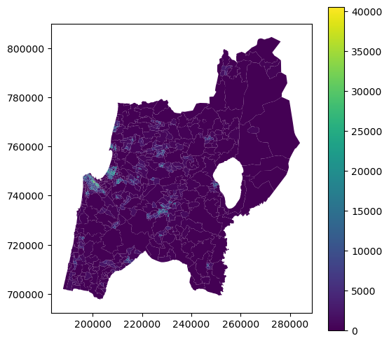

To modify polygon outline style and the color palette, we can use the following additional arguments:

• edgecolor='black'—Black lines
• linewidth=0.1—Reduced line width
• cmap='Reds—The Reds color palette (from colorbrewer)

pol.plot(
    column='POP_DENSE', 
    legend=True,
    edgecolor='black', 
    linewidth=0.1, 
    cmap='Reds'
);

To display more than one layer in the same plot, we need to:

• store the first plot in a variable (e.g., base), and
• pass it as the ax argument of any subsequent plot(s) (e.g., ax=base).

For example:

base = pol.plot(color='red', edgecolor='none')
pnt.plot(ax=base, markersize=0.5, color='black');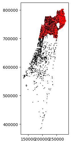

Another useful method to interactively examine the layer(s) is .explore. This creates an interactive map, with a background basemap for context. The parameters of .explore are mostly similar to .plot, with some differences (such as style_kwds for style settings):

pol.explore(
    column='POP_DENSE', 
    legend=True, 
    cmap='Reds',
    style_kwds={'color': 'black', 'weight': 1, 'fillOpacity': 0.5}
)

Make this Notebook Trusted to load map: File -> Trust Notebook

For more information about mapping with geopandas, see the Mapping and Plotting Tools tutorial.

2.5 Geoprocessing

geopandas provides the standard geoprocessing operators, using shapely and pyproj under the hood (which in turn are interfaces to the GEOS and PROJ software, respectively). For example:

• CRS and reprojection—Transforming a given layer from one CRS to another
• Numeric calculations—Calculating numeric geometry properties, such as length, area, and distance
• New geometries—Creating new geometries, such as calculating buffers, or area of intersection
• Geometric relations—Evaluating the relation between layers, such as whether two geometries intersect
• Spatial join—Joining attributes from one layer to another, based on spatial relations

For example, the .area property gives the area sizes of the geometries in CRS units (\(m^2\)):

pol.area

0      6.910450e+06
1      1.774185e+07
2      1.788676e+07
           ...     
778    6.528099e+05
779    5.783374e+05
780    1.073744e+07
Length: 781, dtype: float64

As a more complicated example, let us calculate the distances between each polygon in pol and one point in pnt (Haifa). First, we subset the pnt feature (Haifa) we are interested in, through “selection by attributes”. The GeoDataFrame named haifa has one feature:

haifa = pnt[pnt['שם יישוב'] == 'חיפה']
haifa

	שם יישוב	סמל יישוב	תעתיק	...	x	y	geometry
544	חיפה	4000	HAIFA	...	201120.0	745440.0	POINT (201120.000 745440.000)

1 rows × 26 columns

From that feature, we can extract the first (and only) “geometry”. This is a shapely object, which by default is plotted:

haifa['geometry'].iloc[0]

Now that we have:

• a vector layer (pol), and
• an individual geometry (haifa['geometry'].iloc[0]),

we can use the .distance method to calculate the distances from all polygons to the point. The result is a numeric Series, which we can immediately “insert” as a new attribute named "dist" in pol:

pol['dist'] = pol.distance(haifa['geometry'].iloc[0])
pol

	OBJECTID	POP_DENSE	SHAPE_Leng	...	TAZ_AREA	geometry	dist
0	1	1425.666870	13215.852473	...	6.910450e+06	POLYGON ((217434.341 73558...	17556.437003
1	2	154.888062	21350.948435	...	1.774185e+07	POLYGON ((215109.748 73483...	14726.885602
2	3	115.392609	20113.127398	...	1.788676e+07	POLYGON ((212411.866 74531...	6678.954051
...	...	...	...	...	...	...	...
778	779	10459.399414	4026.527360	...	6.528099e+05	POLYGON ((227634.472 72406...	33459.684072
779	780	1758.489014	3316.818207	...	5.783374e+05	POLYGON ((226951.788 72387...	33493.912906
780	781	518.559326	20705.740930	...	1.073744e+07	POLYGON ((226132.518 72486...	31011.148069

781 rows × 8 columns

Plotting the resulting "dist" attribute shows the distribution of distances, which are between \(0\) and \(80,000\) \(m\) (i.e., \(80\) \(km\)):

base = pol.plot(column='dist', legend=True, cmap='Spectral')
haifa.plot(ax=base, color='blue', edgecolor='black', markersize=80);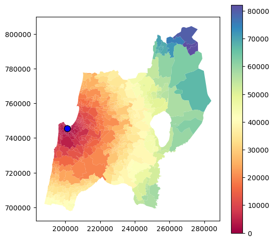

2.6 Writing to file

To export a GeoDataFrame to a vector layer file, we use the .to_file method. The file format is automatically determined according to the chosen file extension, such as:

• .shp—Shapefile
• .gpkg—GeoPackage
• .geojson—GeoJSON

For example, here is how we can export the pol layer to a GeoPackage file named pol.gpkg:

pol.to_file('pol.gpkg')

Figure 2.3 shows the expored file when opened in QGIS.

Figure 2.3: Exported GeoPackage (.gpkg) file viewed in QGIS

2.7 More information

See the Introduction to GeoPandas tutorial (Figure 2.4), and other sections in the geopandas documentation, for more information about geopandas.

Figure 2.4: The Introduction to GeoPandas tutorial