Chapter 4 Tables, conditionals and loops

Last updated: 2023-10-17 21:41:03

Aims

Our aims in this chapter are:

Learn to work with data.frame, the data structure used to represent tables in R
Learn several automation methods for controlling code execution and automation in R:
- Conditionals
- Loops
- The apply function
Learn how to join tables

4.1 Tables

4.1.1 What is a `data.frame`?

A table in R is represented using the data.frame class. A data.frame is basically a collection of vectors comprising columns, all of the same length, but possibly of different types. The convention, in R and elsewhere, is that:

Each table row represents an observation, with values possibly of a different type for each variable
Each table column represents a variable, with values of the same type

For example, the file rainfall.csv, which we are going to work with later on (Section 4.4), contains a table with information about meteorological stations in Israel (Figure 4.1). The table rows correspond to 169 meteorological stations. The table columns refer to different variables:

num—Station ID
altitude—Station altitude above sea level (meters)
sep, oct, …, may—Average rainfall amount in months September, October, …, May, based on the period 1980-2010 (millimeters)
name—Station name
x_utm—X coordinate, in the UTM coordinate system
y_utm—Y coordinate, in the UTM coordinate system

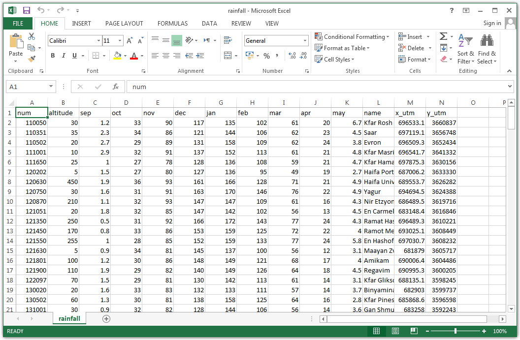
Figure 4.1: rainfall.csv opened in Excel

Note how the data type is the same within each individual column, but possibly different in different columns. For example, the 'altitude' column (elevation above sea level, in meters) contains numeric data, yet the 'name' column (station name) contains textual data. This convention corresponds to the structure of a data.frame in R, as we will see below.

4.1.2 Creating a `data.frame`

A data.frame can be created with the data.frame function, given one or more vectors which become columns. For example, the following expression creates a table with four properties for three railway stations in Israel. The properties are:

name—Station name
city—The city where the station is located
lines—The number of railway lines that go through the station
piano—Does the station have a piano?

dat = data.frame(
    name = c('Beer-Sheva Center', 'Beer-Sheva University', 'Dimona'),
    city = c('Beer-Sheva', 'Beer-Sheva', 'Dimona'),
    lines = c(4, 5, 1),
    piano = c(FALSE, TRUE, FALSE)
)
dat
##                    name       city lines piano
## 1     Beer-Sheva Center Beer-Sheva     4 FALSE
## 2 Beer-Sheva University Beer-Sheva     5  TRUE
## 3                Dimona     Dimona     1 FALSE

Note that, in the above expression, the vectors that comprise the data.frame columns were created inside the function call. Alternatively, we can pass existing vectors to data.frame. For example, the following expression creates the same data.frame as above, this time using pre-defined vectors:

name = c('Beer-Sheva Center', 'Beer-Sheva University', 'Dimona')
city = c('Beer-Sheva', 'Beer-Sheva', 'Dimona')
lines = c(4, 5, 1)
piano = c(FALSE, TRUE, FALSE)
dat = data.frame(name, city, lines, piano)
dat
##                    name       city lines piano
## 1     Beer-Sheva Center Beer-Sheva     4 FALSE
## 2 Beer-Sheva University Beer-Sheva     5  TRUE
## 3                Dimona     Dimona     1 FALSE

4.1.3 Interactive view of a `data.frame`

The View function opens an interactive view of a data.frame. When using RStudio, the view also has sort and filter buttons (Figure 4.2). Note that sorting or filtering the view have no effect on the actual object.

View(dat)

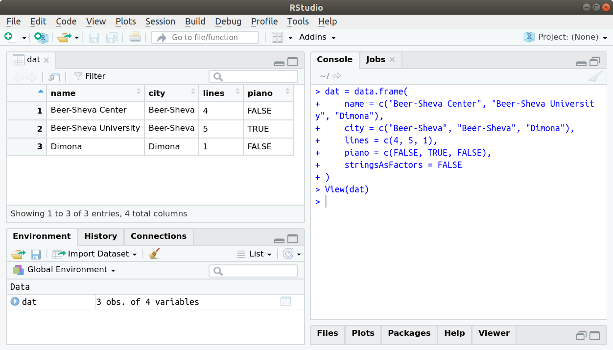
Figure 4.2: Table view in Rstudio

4.1.4 `data.frame` properties

4.1.4.1 Dimensions

Unlike a vector, which is one-dimensional—where the number of elements is obtained with length (Section 2.3.4)—a data.frame is two-dimensional. In R, table rows are considerd the 1^st dimension, while table columns are considered the 2^nd dimension. We can get the number of rows and number of columns in a data.frame with nrow and ncol, respectively:

nrow(dat)
## [1] 3

ncol(dat)
## [1] 4

As an alternative, we can get both the number of rows and columns (in that order!), as a vector of length 2, with dim:

dim(dat)
## [1] 3 4

4.1.4.2 Row and column names

Any data.frame object also has row and column names, which we can get with rownames and colnames, respectively. Row names are usually meaningless, e.g., composed of consecutive numbers by default:

rownames(dat)
## [1] "1" "2" "3"

Conversely, column names are usually meaningful variable names:

colnames(dat)
## [1] "name"  "city"  "lines" "piano"

We can also set row or column names by assigning new values to these properties, or to subsets thereof. For example, here is how we can change the first column name from 'name' to 'STATION_NAME':

colnames(dat)[1] = 'STATION_NAME'
dat
##            STATION_NAME       city lines piano
## 1     Beer-Sheva Center Beer-Sheva     4 FALSE
## 2 Beer-Sheva University Beer-Sheva     5  TRUE
## 3                Dimona     Dimona     1 FALSE

and revert it back to 'name':

colnames(dat)[1] = 'name'
dat
##                    name       city lines piano
## 1     Beer-Sheva Center Beer-Sheva     4 FALSE
## 2 Beer-Sheva University Beer-Sheva     5  TRUE
## 3                Dimona     Dimona     1 FALSE

The str function gives a summary of any object structure. For data.frame objects, str lists the dimensions, as well as column names, types and (first few) values in each column:

str(dat)
## 'data.frame':    3 obs. of  4 variables:
##  $ name : chr  "Beer-Sheva Center" "Beer-Sheva University" "Dimona"
##  $ city : chr  "Beer-Sheva" "Beer-Sheva" "Dimona"
##  $ lines: num  4 5 1
##  $ piano: logi  FALSE TRUE FALSE

4.1.5 `data.frame` subsetting

4.1.5.1 Introduction

A data.frame subset can be obtained with the [ operator, which we are familiar with from vector subsetting (Sections 2.3.3 and 2.3.8). Since a data.frame is a two-dimensional object, the data.frame subsetting method accepts two vectors:

The first vector refers to rows
The second vector refers to columns

Each of these vectors can be one of the following types:

numeric—Specifying the indices of rows/columns to retain
character—Specifying the names of rows/columns to retain
logical—Specifying whether to retain each row/column

Either the rows or the column index can be omitted, in which case we get all rows or all columns, respectively. The following Sections 4.1.5.2–4.1.5.5 give examples of the three data.frame subsetting methods.

4.1.5.2 Numeric index

Here are several examples of subsetting with a numeric index:

dat[1, 1]        # Row 1, column 1
## [1] "Beer-Sheva Center"

dat[c(1, 3), 2]  # Rows 1 & 3, column 2
## [1] "Beer-Sheva" "Dimona"

dat[2, ]         # Row 2
##                    name       city lines piano
## 2 Beer-Sheva University Beer-Sheva     5  TRUE

dat[, 2:1]       # Columns 2 & 1
##         city                  name
## 1 Beer-Sheva     Beer-Sheva Center
## 2 Beer-Sheva Beer-Sheva University
## 3     Dimona                Dimona

As you may have noticed based on the way the output is printed, the first two expressions return a (character) vector, while the last two expressions return a data.frame (check using the class function!). Section 4.1.5.3 describes how the type of returned subset is determined, and how it can be controlled using the drop parameter.

4.1.5.3 The `drop` parameter

The subset operator [ accepts an additional logical argument drop. The drop argument determines whether we would like to simplify the resulting subset to a simpler data structure, when possible, “dropping” the more complex class (drop=TRUE, the default), or whether we would like to always keep the subset in its original class (drop=FALSE).

When applied to a data.frame, a subset that contains a single data.frame column can be returned as:

A vector (drop=TRUE, the default)
A data.frame (drop=FALSE)

A subset that contains two or more columns is returned as a data.frame, regardless of the drop argument value.

In other words, we need to use drop=FALSE in case we want to make sure that the subset is returned as a data.frame no matter what. Otherwise, a subset composed of a single column is returned as a vector.

For example, a subset that contains a single column is, by default, simplified to a vector:

dat[1:2, 1]
## [1] "Beer-Sheva Center"     "Beer-Sheva University"

unless we specify drop=FALSE, in which case it remains a data.frame:

dat[1:2, 1, drop = FALSE]
##                    name
## 1     Beer-Sheva Center
## 2 Beer-Sheva University

Why do you think simplification works when taking a subset with a single column, but not on a subset with a single row?

4.1.5.4 Character index

We can also use a character index to specify the names of rows and/or columns to retain in the subset. A character index is mostly useful for subsetting columns, where names are meaningful (Section 4.1.4.2). For example:

dat[, 'name']
## [1] "Beer-Sheva Center"     "Beer-Sheva University" "Dimona"

dat[, c('name', 'city')]
##                    name       city
## 1     Beer-Sheva Center Beer-Sheva
## 2 Beer-Sheva University Beer-Sheva
## 3                Dimona     Dimona

The $ operator is a shortcut for getting a single column, by name, from a data.frame:

dat$name
## [1] "Beer-Sheva Center"     "Beer-Sheva University" "Dimona"

dat$city
## [1] "Beer-Sheva" "Beer-Sheva" "Dimona"

4.1.5.5 Logical index

The third option for a data.frame index is a logical vector, specifying whether to retain each row or column. Most often, a logical vector index is used to filter data.frame rows, based on the values of one or more columns. For example:

dat[dat$city == 'Beer-Sheva', ]
##                    name       city lines piano
## 1     Beer-Sheva Center Beer-Sheva     4 FALSE
## 2 Beer-Sheva University Beer-Sheva     5  TRUE

dat[dat$piano, ]
##                    name       city lines piano
## 2 Beer-Sheva University Beer-Sheva     5  TRUE

dat[dat$city == 'Beer-Sheva' & !dat$piano, ]
##                name       city lines piano
## 1 Beer-Sheva Center Beer-Sheva     4 FALSE

What is the meaning of the above three expressions, in plain language?

Let’s go back to the Kinneret example from Chapter 3. To do that, we once again define the two vectors time and value:

value = c(-211.92, -212.79, -208.8, -209.52, -208.84, -209.72, -209.12, 
-210.94, -209.01, -210.85, -209.60, -211.40, -210.24, -212.01, 
-210.46, -212.25, -211.76, -213.00, -211.92, -213.71, -213.13, -214.78, 
-213.18, -214.34, -209.74, -210.93, -208.92, -210.69, -209.73, 
-211.64, -210.68, -212.03, -211.1, -212.60, -212.18, -214.23, 
-213.26, -214.33, -212.65, -213.89, -212.37, -213.68)
time = rep(1991:2011, each = 2)
time = paste0(time, c('-05-15', '-11-15'))
time = as.Date(time)

Now, we already know how to combine the vectors into a data.frame (Section 4.1.2), using the data.frame function. The following expression combines time and value into a data.frame named kineret:

kineret = data.frame(time, value)

This is a longer table than the previous one, so printing all of it is inconvenient as it takes a lot of space in the console. Instead, we can use the head or tail functions, which return a subset of the first or last six rows of a data.frame, respectively. This is usually sufficient to understand the structure of the data.frame:

head(kineret)
##         time   value
## 1 1991-05-15 -211.92
## 2 1991-11-15 -212.79
## 3 1992-05-15 -208.80
## 4 1992-11-15 -209.52
## 5 1993-05-15 -208.84
## 6 1993-11-15 -209.72

tail(kineret)
##          time   value
## 37 2009-05-15 -213.26
## 38 2009-11-15 -214.33
## 39 2010-05-15 -212.65
## 40 2010-11-15 -213.89
## 41 2011-05-15 -212.37
## 42 2011-11-15 -213.68

Using a logical index, we can get a subset of dates when the Kinneret level was less than -213.2. Note that the following expression is identical to the one we used when working with separate vectors time and value (Section 3.1.4), except for the kineret$ part, which now specifies that we refer to data.frame columns:

kineret$time[kineret$value < -213.2]
## [1] "2000-11-15" "2001-11-15" "2002-11-15" "2008-11-15" "2009-05-15"
## [6] "2009-11-15" "2010-11-15" "2011-11-15"

When operating on a data.frame, we can also get a subset with data from all columns for the dates of interest, as follows:

kineret[kineret$value < -213.2, ]
##          time   value
## 20 2000-11-15 -213.71
## 22 2001-11-15 -214.78
## 24 2002-11-15 -214.34
## 36 2008-11-15 -214.23
## 37 2009-05-15 -213.26
## 38 2009-11-15 -214.33
## 40 2010-11-15 -213.89
## 42 2011-11-15 -213.68

What are the differences between the last two expressions? What is the reason for those differences?

4.1.6 Creating new columns

Assignment into a data.frame column which does not yet exist adds a new column. For example, here is how we can add a new column named d_nov, containing differences between consecutive values in the nov column (Section 3.1.5):

kineret$d_value = c(NA, diff(kineret$value))

We now have a new (third) column in the data.frame, with the consecutive water level differences:

head(kineret)
##         time   value d_value
## 1 1991-05-15 -211.92      NA
## 2 1991-11-15 -212.79   -0.87
## 3 1992-05-15 -208.80    3.99
## 4 1992-11-15 -209.52   -0.72
## 5 1993-05-15 -208.84    0.68
## 6 1993-11-15 -209.72   -0.88

4.2 Flow control

4.2.1 Overview

The default execution mode is to let the computer execute all expressions in the same order they are given in the code. Flow control commands are a way to modify the sequence of code execution. We will learn two flow control operators, from two flow control categories:

if and else—A conditional, conditioning the execution of code
for—A loop, executing code more than once

4.2.2 Conditionals

The purpose of the conditional is to condition the execution of code. An if/else conditional in R contains the following components:

The if keyword
A condition, inside parentheses (( and ))
Code to be executed if the condition is TRUE, inside curly brackets ({ and })
The else keyword (optional)
Code to be executed if the condition is FALSE, inside curly brackets ({ and }) (optional)

The condition must be evaluated to a logical vector of length 1, containing either TRUE or FALSE. If the condition is TRUE, then the code section after if is executed. If the condition is FALSE, then the code section after else (when present) is executed.

Here is the syntax of a conditional with if:

if(condition) {
  expressions
}

and here is the syntax of a conditional with both if and the optional else:

if(condition) {
  true_expressions
} else {
  false_expressions
}

The following examples demonstrate how the expression after if is executed when the condition is TRUE:

x = 3
if(x > 0) print('x is positive!')
## [1] "x is positive!"

Note that the curly brackets ({ and }) are omitted, because the code section contains one expression only, same as in a function definition (Section 3.3.4).

When the condition is FALSE—nothing happens:

x = -5
if(x > 0) print('x is positive!')

Now let’s also add a second expression after else. The first code section is still executed when the condition is TRUE:

x = 3
if(x > 0) print('x is positive!') else print('x is negative or zero!')
## [1] "x is positive!"

When the condition is FALSE, however, the second code section is executed instead:

x = -5
if(x > 0) print('x is positive!') else print('x is negative or zero!')
## [1] "x is negative or zero!"

How can the above conditional expression be expanded to print one of three messages, indicating whether x is positive, negative, or zero?

Conditionals are frequently used when our code branches into two (or more) scenarios, depending on the value of a particular object. For example, we can use a conditional to define (Section 3.3) our own version of the abs function (Section 2.3.4):

abs2 = function(x) {
  if(x < 0) return(-x) else return(x)
}

Let’s check if our custom function abs2 works as expected:

abs2(-3)
## [1] 3

abs2(0)
## [1] 0

abs2(24)
## [1] 24

It does (for vectors of length 1!).

4.2.3 Loops

A loop is used to execute a given code section more than once. The number of times the code is executed is determined in different ways in different types of loops. In a for loop, the number of times the code is executed is determined in advance, based on the length of a vector passed when the loop is initialized. The code is executed once for each element of the vector. In each “round”, the current element is assigned to a variable, which we can use in the loop code.

A for loop is composed of the following parts:

The for keyword
The variable name which we assign to the current vector element (symbol)
The in keyword
The vector we go over (sequence)
A code section which defines what to do with each element (expressions)

Here is the syntax of a for loop:

for(symbol in sequence) {
  expressions
}

Note that the constant keywords are just for and in. All other components—namely, symbol, sequence and expressions—are varying, and it is up to us to choose their values.

Here is an example of a for loop:

for(i in 1:5) print(i)
## [1] 1
## [1] 2
## [1] 3
## [1] 4
## [1] 5

What has happened? The expression print(i) was executed 5 times, according to the length of the vector 1:5. Each time, i got the next value of 1:5 and the code section printed that value on screen.

The vector defining the for loop does not necessarily need to be numeric. For example:

for(b in c('Test', 'One', 'Two')) print(b)
## [1] "Test"
## [1] "One"
## [1] "Two"

Here, the expression print(b) was executed 3 times, according to the length of the vector c('Test','One','Two'). Each time, b got the next value of the vector and the code section printed b on screen.

In case the vector is numeric, it does not necessarily need to be composed of consecutive values:

for(i in c(8,15,3)) print(i)
## [1] 8
## [1] 15
## [1] 3

Again, the expression print(i) was executed 3 times, now according to the length of the vector c(8,15,3). Each time, i got the next value of the vector and the code section printed i on screen.

The code section even does not have to use the current value of the vector:

for(i in 1:5) print('A')
## [1] "A"
## [1] "A"
## [1] "A"
## [1] "A"
## [1] "A"

Here, the expression print('A') was executed 5 times, according to the length of the vector 1:5. Each time, the code section printed the fixed value 'A' on screen.

The following for loop prints each of the numbers from 1 to 10 multiplied by 5:

for(i in 1:10) print(i * 5)
## [1] 5
## [1] 10
## [1] 15
## [1] 20
## [1] 25
## [1] 30
## [1] 35
## [1] 40
## [1] 45
## [1] 50

How can we print ten vectors of lenght 10, comprising a multiplication table for 1-10, using a for loop?

##  [1]  1  2  3  4  5  6  7  8  9 10
##  [1]  2  4  6  8 10 12 14 16 18 20
##  [1]  3  6  9 12 15 18 21 24 27 30
##  [1]  4  8 12 16 20 24 28 32 36 40
##  [1]  5 10 15 20 25 30 35 40 45 50
##  [1]  6 12 18 24 30 36 42 48 54 60
##  [1]  7 14 21 28 35 42 49 56 63 70
##  [1]  8 16 24 32 40 48 56 64 72 80
##  [1]  9 18 27 36 45 54 63 72 81 90
##  [1]  10  20  30  40  50  60  70  80  90 100

As another example of using a for loop, we can write a function named x_in_y. The function accepts two vectors x and y. For each element in x the function checks whether it is found in y. It returns a logical vector of the same length as x.

Here is an example of how the function is supposed to work:

x = c(1, 2, 3, 4, 5)
y = c(2, 1, 5, 5)
x_in_y(x, y)
## [1]  TRUE  TRUE FALSE FALSE  TRUE

In plain terms, we need to go over the elements of x, each time checking whether the current element is equal to any of the elements in y. What may first come to mind is the expression:

x == y
## Warning in x == y: longer object length is not a multiple of shorter object
## length
## [1] FALSE FALSE FALSE FALSE FALSE

However, this is not the right answer. Remember that comparing two vectors with == returns a pairwise vector of results (Section 2.3.10). What we need is to compare each element of x to all elements of y. Translating to R code, here is what we need to do:

c(
  any(x[1] == y),
  any(x[2] == y),
  any(x[3] == y),
  any(x[4] == y),
  any(x[5] == y)
)
## [1]  TRUE  TRUE FALSE FALSE  TRUE

The last code section makes long code and is not very general: it depends on the length of x. This is exactly the type of operation where a for loop comes in handy. We can use a for loop to check if each element in x is contained in y, as follows:

for(i in x) print(any(i == y))
## [1] TRUE
## [1] TRUE
## [1] FALSE
## [1] FALSE
## [1] TRUE

Inside the function, rather then just printing, we would like to “collect” the results into a vector that will be returned to the user. To do that, we can start from a vector composed of NA with the right length (rep(NA,length(x))), then fill-in the results using assignment. Note that the for loop needs to be different, for(i in 1:length(x)) instead of for(i in x), so that we have access to both the indices i and the values x[i]:

for(i in 1:length(x)) print(any(x[i] == y))
## [1] TRUE
## [1] TRUE
## [1] FALSE
## [1] FALSE
## [1] TRUE

In the first for loop version, we go over the elements of x, therefore the loop is initialized with for(i in x). In the second version, we go over the indices of x, therefore the loop is initialized with for(i in 1:length(x)).

Here is the entire code of the function:

x_in_y = function(x, y) {
  result = rep(NA, length(x))
  for(i in 1:length(x)) result[i] = any(x[i] == y)
  result
}

Note the difference in the for loop vector that we go over in the two versions.

Execute the above function definition and then the specific example shown earlier to demonstrate that the x_in_y function works properly.

What change(s) do we need to make in the x_in_y function to create a new function named times_x_in_y, which returns the count of occurences in y for each element in x, as shown below?

times_x_in_y(x, y)
## [1] 1 1 0 0 2

Situations when we need to go over subsets of a dataset, process those subsets, then combine the results back to a single object, are very common in data processing. A for loop is the default approach for such tasks, unless there is a “shortcut” that we may prefer, such as the apply function (Section 4.5). For example, we will come back to for loops when separately processing raster layers for several time periods (Section 11.3.2).

4.3 The `%in%` operator

In fact, we don’t need to write a function such as x_in_y (Section 4.2.3) ourselves. The functionality already exists in R, in the form of an operator called %in%. The %in% operator, in an expression x %in% y, returns a logical vector indicating the presence of each element of x in y. For example:

1:5 %in% c(1, 2, 5)
## [1]  TRUE  TRUE FALSE FALSE  TRUE

Keep in mind that the order of arguments of the %in% operator matters. Namely, we are evaluating the presence of the left-side vector in the right-side vector. Therefore, the following expression has a different meaning:

c(1, 2, 5) %in% 1:5
## [1] TRUE TRUE TRUE

Here are two more examples using %in% with the letters and LETTERS built-in vectors. (Type the names of these two vectors to see what they are).

c('a', 'B', 'c', 'ee') %in% letters
## [1]  TRUE FALSE  TRUE FALSE

c('a', 'B', 'c', 'ee') %in% LETTERS
## [1] FALSE  TRUE FALSE FALSE

4.4 Reading tables from a file

4.4.1 Using `read.csv`

In addition to creating a table with data.frame (Section 4.1.2), we can read an existing table from a file, such as from a Comma-Separated Values (CSV) file¹⁴. This operation creates a data.frame object with file contents in the RAM (Figure 4.3).

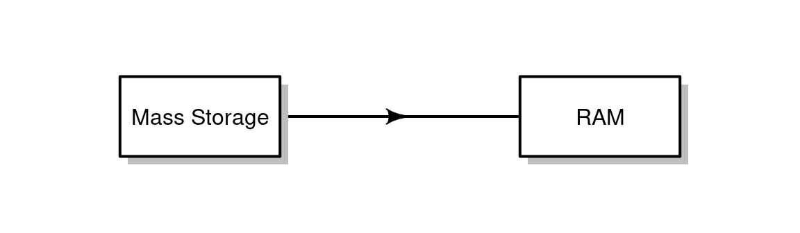
Figure 4.3: Reading a file takes information from the Mass Storage and loads it into the RAM.

In the next few examples in this chapter, we will work with the CSV file named rainfall.csv (Figure 4.1). This file contains a table with average monthly (September–May) rainfall data, based on the period 1980-2010, in 169 meteorological stations in Israel. The table also contains station name, number, elevation above sea level, and X-Y coordinates.

We can read a CSV file using the read.csv function, given the file path. For example, assuming the file rainfall.csv is located in the C:\Data2 directory, we can read it using either of the following two expressions:

read.csv('C:\\Data2\\rainfall.csv')
read.csv('C:/Data2/rainfall.csv')

Note that the valid separating character is either / or \\ (not the familiar \!). In case the file path uses the incorrect separator \, we get an error:

read.csv('C:\Data2\rainfall.csv')
## Error: '\D' is an unrecognized escape in character string (<text>:1:14)

In case the path is correct but the requested file does not exist, we also get an error, but a different one:

read.csv('C:\\Data2\\rainfall.csv')
## Warning in file(file, "rt"): cannot open file 'C:\Data2\rainfall.csv': No such
## file or directory
## Error in file(file, "rt"): cannot open the connection

When using the right path separator and a path to an existing file, reading should be successful, in which case a new data.frame is created in the R environment.

4.4.2 The working directory

When reading files into R, there is another important concept we need to be aware of: the working directory. The R environment always points to a certain directory on our computer, which is known as the working directory. We can get the current working directory with getwd:

getwd()
## [1] "/home/michael/Sync/courses2/r_2023/book"

We can set a different working directory with setwd:

setwd('C:\\Data2')

When reading a file from the working directory, we can specify just the file name, instead of the full path:

read.csv('rainfall.csv')

We can also specify a relative file path, starting from the working directory. For example, the following expression reads the rainfall.csv file from the directory named data which is in the working directory:

read.csv('data/rainfall.csv')

This is the convention we are going to use in all of the book examples. If you want to run the code examples as-is, you need to download the sample data files (Appendix A), then place them in a directory named data inside your working directory (or change the working directory to where the data directory is).

When reading and/or writing multiple files from the same directory, it is convenient to set the working directory at the beginning of our script. That way, in the rest of our script, we can refer to the various files by file name only, rather than by the full path.

The best-practice, however, is trying to avoid specifying a working directory, or any other machine-specific file paths, altogether. Instead, we prefer to assume that the working directory is where the code file is. That way, the code is made as reproducible as possible.

4.4.3 Example: the `rainfall.csv` dataset

Let’s read the rainfall.csv file into a data.frame object named rainfall:

rainfall = read.csv('rainfall.csv')

We can check the table structure with str, as shown previously (Section 4.1.4.2), to see the dimensions, column names, columns data types, and the first few values in each column:

str(rainfall)
## 'data.frame':    169 obs. of  14 variables:
##  $ num     : int  110050 110351 110502 111001 111650 120202 120630 120750 120870 121051 ...
##  $ altitude: int  30 35 20 10 25 5 450 30 210 20 ...
##  $ sep     : num  1.2 2.3 2.7 2.9 1 1.5 1.9 1.6 1.1 1.8 ...
##  $ oct     : int  33 34 29 32 27 27 36 31 32 32 ...
##  $ nov     : int  90 86 89 91 78 80 93 91 93 85 ...
##  $ dec     : int  117 121 131 137 128 127 161 163 147 147 ...
##  $ jan     : int  135 144 158 152 136 136 166 170 147 142 ...
##  $ feb     : int  102 106 109 113 108 95 128 146 109 102 ...
##  $ mar     : int  61 62 62 61 59 49 71 76 61 56 ...
##  $ apr     : int  20 23 24 21 21 19 21 22 16 13 ...
##  $ may     : num  6.7 4.5 3.8 4.8 4.7 2.7 4.9 4.9 4.3 4.5 ...
##  $ name    : chr  "Kfar Rosh Hanikra" "Saar" "Evron" "Kfar Masrik" ...
##  $ x_utm   : num  696533 697119 696509 696542 697875 ...
##  $ y_utm   : num  3660837 3656748 3652434 3641332 3630156 ...

Create a plot of rainfall in January (jan) as function of elevation (altitude) based on the rainfall table (Figure 4.4).

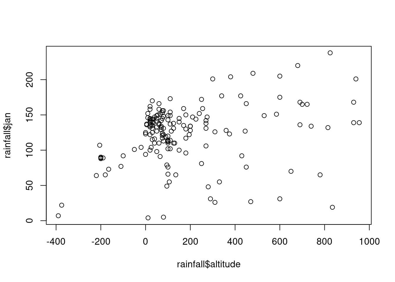
Figure 4.4: Rainfall amount in January as function of elevation

We can get specific information from the table trough subsetting and summarizing. For example, what are the elevations of the lowest and highest stations?

min(rainfall$altitude)
## [1] -390

max(rainfall$altitude)
## [1] 955

What are the names of the lowest and highest stations?

rainfall$name[which.min(rainfall$altitude)]
## [1] "Sdom"

rainfall$name[which.max(rainfall$altitude)]
## [1] "Rosh Tzurim"

How much rainfall does the 'Haifa University' station receive in April?

We can create a new column using assignment (Section 4.1.6). For example, here is how we can create a new column named sep_oct, with the amounts of rainfall in September and October combined:

rainfall$sep_oct = rainfall$sep + rainfall$oct

If we want to remove a column, we can assign NULL (Section 1.3.5) to it:

rainfall$sep_oct = NULL

To accomodate more complex calculations, we can also “build” a new column inside a for loop, going over table rows. For example, the following code section calculates a new column named annual, with the total annual precipitation amounts per station:

m = c('sep', 'oct', 'nov', 'dec', 'jan', 'feb', 'mar', 'apr', 'may')
rainfall$annual = NA
for(i in 1:nrow(rainfall)) {
  rainfall$annual[i] = sum(rainfall[i, m])
}

Note that the annual column is first initialized with NA (which is recycled to fill the entire column). Inside the for loop, the annual column is then filled with the calculated rainfall sums. Note how the sum function is applied on a (numeric!) subset of data.frame rows and columns, treating it the same way as a numeric vector, using the expression sum(rainfall[i,m]).

Go over the above code and make sure you understand how it works.

The updated rainfall table with the new columns is shown below:

head(rainfall)
##      num altitude sep oct nov dec jan feb mar apr may              name
## 1 110050       30 1.2  33  90 117 135 102  61  20 6.7 Kfar Rosh Hanikra
## 2 110351       35 2.3  34  86 121 144 106  62  23 4.5              Saar
## 3 110502       20 2.7  29  89 131 158 109  62  24 3.8             Evron
## 4 111001       10 2.9  32  91 137 152 113  61  21 4.8       Kfar Masrik
## 5 111650       25 1.0  27  78 128 136 108  59  21 4.7     Kfar Hamakabi
## 6 120202        5 1.5  27  80 127 136  95  49  19 2.7        Haifa Port
##      x_utm   y_utm annual
## 1 696533.1 3660837  565.9
## 2 697119.1 3656748  582.8
## 3 696509.3 3652434  608.5
## 4 696541.7 3641332  614.7
## 5 697875.3 3630156  562.7
## 6 687006.2 3633330  537.2

4.5 The `apply` function

In the last example (Section 4.4.3), we used a for loop to apply a function (sum) on each and every row of a table (rainfall[,m]). The apply function can replace for loops in such situations, and more generally: in situations when we are interested in applying the same function on all subsets of certain dimension of a data.frame (see below), a matrix (Section 5.1.8), or an array (Section 5.2.3).

In case of a data.frame, there are two dimensions that we can work on with apply:

Rows = Dimension 1
Columns = Dimension 2

Given the dimension of choice, and a function, apply splits the table into separate rows or columns, applies the function, and combines the results back into a complete object (Figure 4.5). Accordingly, the set of techniques which apply belongs to is known as split-apply-combine (Wickham et al. 2011).

Figure 4.5: The apply function, applying the mean function on rows (left) or columns (right). This figure is from Murrell (2009).

The apply function needs three arguments:

X—The object we are working on: data.frame, matrix (Section 5.1.8), or array (Section 5.2.3)
MARGIN—The dimension(s) we are working on
FUN—The function applied on each subset(s)

For example, the apply function can be used, instead of a for loop, to calculate the total annual rainfall per station. To do that, we apply the sum function on the rows dimension:

rainfall$annual = apply(X = rainfall[, m], MARGIN = 1, FUN = sum)

or, in short:

rainfall$annual = apply(rainfall[, m], 1, sum)

As another example, we can calculate average monthly rainfall, across all 169 stations, for each month. This time, the mean function is applied on the columns dimension:

avg_rain = apply(rainfall[, m], 2, mean)

The result avg_rain is a named numeric vector. Element names correspond to column names of rainfall[,m]:

avg_rain
##        sep        oct        nov        dec        jan        feb        mar 
##   1.025444  21.532544  64.852071 105.798817 123.053254 103.130178  58.366864 
##        apr        may 
##  16.769231   3.968639

For most purposes, such as when applying arithmetic or logical operators, a named vector behaves exactly the same way as an ordinary (unnamed) vector. However, there are some situations where the vector names come into play. For example, we can quickly visualize the values of a named vector using the barplot function, which displays the vector names on the x-axis and the vector values on the y-axis (Figure 4.6):

barplot(avg_rain)

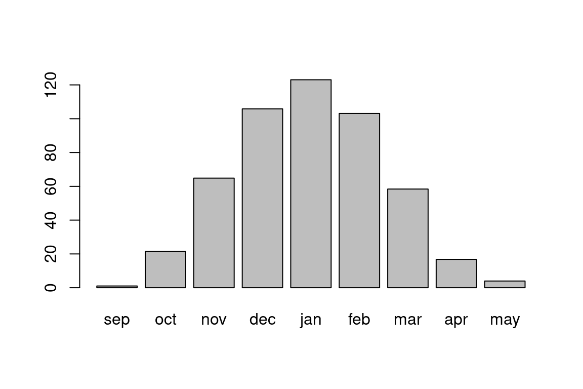
Figure 4.6: Average rainfall per month, among 169 stations in Israel

As another example, let’s use apply to find the station name with the highest rainfall amount, per month. This is a more complicated example, which takes two steps to complete. First, we apply which.max on the columns, returning the row indices where the maximal rainfall values are located, per column:

max_st = apply(rainfall[, m], 2, which.max)
max_st
## sep oct nov dec jan feb mar apr may 
##  71  23  77  77  77  66  66  66  77

Second, we obtain the corresponding station names, by subsetting the name column using the indices we got in the first step:

rainfall$name[max_st]
## [1] "Eilon"      "Maabarot"   "Horashim"   "Horashim"   "Horashim"  
## [6] "Golan Farm" "Golan Farm" "Golan Farm" "Horashim"

It makes sense to combine the final result with the month names, in the form of a table, as follows:

data.frame(month = m, name = rainfall$name[max_st])
##   month       name
## 1   sep      Eilon
## 2   oct   Maabarot
## 3   nov   Horashim
## 4   dec   Horashim
## 5   jan   Horashim
## 6   feb Golan Farm
## 7   mar Golan Farm
## 8   apr Golan Farm
## 9   may   Horashim

The meaning of the result is that in September, the Eilon station has the highest amount of rainfall, the Maabarot station has the highest amount of rainfall in October, etc.

What do we need to change in the above code sections to get a table of stations where the rainfall amount is smallest, per month?

4.6 Table joins

4.6.1 Classification

In the next example, we are going to work with another table, from a CSV file named MOD13A3_2000_2019_dates.csv. The MOD13A3_2000_2019_dates.csv table contains the corresponding dates for each layer in the raster MOD13A3_2000_2019.tif, which is a monthly time series of NDVI images (Figure 5.13). We are going to work with this raster starting from Chapter 5.

Let’s import the table into R, into a data.frame named dates:

dates = read.csv('data/MOD13A3_2000_2019_dates.csv')

Here is what the first few rows in dates look like:

head(dates)
##   layer       date
## 1     1 2000-02-15
## 2     2 2000-03-15
## 3     3 2000-04-15
## 4     4 2000-05-15
## 5     5 2000-06-15
## 6     6 2000-07-15

The table has two columns, layer and date. The layer column contains the raster layer indices, from 1 to 233. The date column contains the dates corresponding to each raster layer. The raster layers comprise a monthly time series, where the layers contain monthly average NDVI values. Therefore, the days in the dates table are arbitrarily set to the 15^th of the respective month.

Later on in this book, we are going to group the raster layers by season (Section 11.3.2), according to the dates. How can we calculate a new season column, classifying each date in the dates table (and later, each image) into the season it belongs to? Our approach will be composed of two parts. First (see below), we are going to extract the month component of each date. Second (Section 4.6.2), we will classify the months into season names, using a table join.

First, we need to figure out the month each date belongs to, which we know how to do from Section 3.1.2. To do that, we transform the date column from character to Date, using as.Date (Section 3.1.2.2). Then, we extract the month from all dates, using the combination of format and as.numeric (Section 3.1.2.3):

dates$date = as.Date(dates$date)
dates$month = format(dates$date, '%m')
dates$month = as.numeric(dates$month)

Now the dates table has an additional month column:

head(dates)
##   layer       date month
## 1     1 2000-02-15     2
## 2     2 2000-03-15     3
## 3     3 2000-04-15     4
## 4     4 2000-05-15     5
## 5     5 2000-06-15     6
## 6     6 2000-07-15     7

Second, we need to classify the months into one of the four seasons, according to the well-known scheme given in Table 4.1.

Table 4.1: Months and seasons
Season	Months
`'winter'`	`12`, `1`, `2`
`'spring'`	`3`, `4`, `5`
`'summer'`	`6`, `7`, `8`
`'fall'`	`9`, `10`, `11`

The most straightforward way to classify the months into seasons, is through a series of assignment to subset operations (Section 2.3.9). Namely, we can assign each season name into the right subset of a new season column, depending on the month:

dates$season = NA
dates$season[dates$month %in% c(12, 1:2)] = 'winter'
dates$season[dates$month %in% 3:5] = 'spring'
dates$season[dates$month %in% 6:8] = 'summer'
dates$season[dates$month %in% 9:11] = 'fall'

Again, note that we first initialize the column with NA values (in the first expression), then replace them (in the last four expressions), much like in the last for loop example (Section 4.4.3).

Here is the result:

head(dates)
##   layer       date month season
## 1     1 2000-02-15     2 winter
## 2     2 2000-03-15     3 spring
## 3     3 2000-04-15     4 spring
## 4     4 2000-05-15     5 spring
## 5     5 2000-06-15     6 summer
## 6     6 2000-07-15     7 summer

This method of classification may be inconvenient when we have many categories or complex criteria. A more general approach is to use a table join, which is what we learn about next (Section 4.6.2).

4.6.2 Joining tables with `merge`

4.6.2.1 Types of table joins

A table join combines rows from two tables into one table, based on identity of values in shared columns. There are several types of joins, such as left, right, inner and full joins, differing in the way that non-matching rows are dealt with (Figure 4.7).

A schematic illustration of join types. The circles represent the two tables being joined, the left and right one. The shaded area represents the returned records; for example, a *left join* returns all records from the left table with the matching records from the right table. The respective `merge` function argument is given in parentheses.

Figure 4.7: A schematic illustration of join types. The circles represent the two tables being joined, the left and right one. The shaded area represents the returned records; for example, a left join returns all records from the left table with the matching records from the right table. The respective merge function argument is given in parentheses.

In this book, we will use just one type of join—known as a left join—which is the most useful type of join. In a left join, given two tables x and y, we get all of the rows of the first table x, with the matching row(s), if any, from y. In case there is no matching row in y for a given row in x, the row is still returned, with all values that were supposed to come from y set as NA¹⁵. Matching rows are determined based on identical values in one or more columns that are common both to x and y.

4.6.2.2 The `merge` function

The merge function can do several types of table joins in R. The first two parameters are the tables that need to be joined, x and y. The third by parameter is the common column name(s) by which the tables need to be joined. When employing a left join, we also specify all.x=TRUE (Figure 4.7). The latter setting means that all rows of x need to be kept in the resulting table, even if they do not have a match in y, which is the definition of a left join.

4.6.2.3 Population in four cities

As a small example of a table join, consider the following table dat2, which contains information about population size of four cities¹⁶:

dat2 = data.frame(
  city = c('Beer-Sheva', 'Haifa', 'Jerusalem', 'Tel-Aviv'),
  population = c(209687, 285316, 936425, 460613)
)
dat2
##         city population
## 1 Beer-Sheva     209687
## 2      Haifa     285316
## 3  Jerusalem     936425
## 4   Tel-Aviv     460613

Here is the merge expression for a left join between the dat and dat2 tables, according to the common 'city' column:

merge(dat, dat2, by = 'city', all.x = TRUE)
##         city                  name lines piano population
## 1 Beer-Sheva     Beer-Sheva Center     4 FALSE     209687
## 2 Beer-Sheva Beer-Sheva University     5  TRUE     209687
## 3     Dimona                Dimona     1 FALSE         NA

What is the difference between the above result and the “left” table dat? Why was the third value in the 'population' column set to NA?

4.6.2.4 Classifying seasons

Let’s get back to the dates table. The table we are going to join with dates is a small table named seasons, which contains the season classifications of the 12 months. We can prepare the seasons table as follows (Section 2.3.6.3):

seasons = data.frame(
  month = c(12, 1:11),
  season = rep(c('winter', 'spring', 'summer', 'fall'), each = 3)
)
seasons
##    month season
## 1     12 winter
## 2      1 winter
## 3      2 winter
## 4      3 spring
## 5      4 spring
## 6      5 spring
## 7      6 summer
## 8      7 summer
## 9      8 summer
## 10     9   fall
## 11    10   fall
## 12    11   fall

Now we can join the dates and seasons tables. Before that, we remove the season column we manually created earlier (Section 4.6.1):

dates$season = NULL
head(dates)
##   layer       date month
## 1     1 2000-02-15     2
## 2     2 2000-03-15     3
## 3     3 2000-04-15     4
## 4     4 2000-05-15     5
## 5     5 2000-06-15     6
## 6     6 2000-07-15     7

Then we use merge to join the tables:

dates = merge(dates, seasons, by = 'month', all.x = TRUE)

Examining the result shows that the season column was indeed joined:

head(dates)
##   month layer       date season
## 1     1    12 2001-01-15 winter
## 2     1    36 2003-01-15 winter
## 3     1    96 2008-01-15 winter
## 4     1    84 2007-01-15 winter
## 5     1    60 2005-01-15 winter
## 6     1    48 2004-01-15 winter

The joined table was automatically sorted by the common column month. It can be sorted back to chronological order using the order function (Section 2.4.4):

dates = dates[order(dates$date), ]
head(dates)
##     month layer       date season
## 20      2     1 2000-02-15 winter
## 40      3     2 2000-03-15 spring
## 60      4     3 2000-04-15 spring
## 81      5     4 2000-05-15 spring
## 104     6     5 2000-06-15 summer
## 122     7     6 2000-07-15 summer

Note that that, as a result of the join, the order of the first there columns also changed. How can we get back to the original order of the first three columns?

4.7 Writing tables to file

To keep a data.frame we calculated in persistent storage, for later use, we need to export it to a file. For example, we may wish to export the the modified dates table, which now has a 'season' column (Section 4.6.2). That way, for example, we can import the table in other R code files for further processing, send it to colleagues, import and view it in other software (such as Excel), and so on.

The write.csv function can be used to write the contents of a data.frame to a CSV file (Figure 4.8). This may be considered as the opposite of read.csv (Section 4.4). The most important parameters of read.csv are:

The data.frame we want to export
The file name, or file path, of the CSV file we want to create
row.names—Whether to export row names or not (default is TRUE)

For example, here is how we write the dates table into a file named MOD13A3_2000_2019_dates2.csv in our working directory:

write.csv(dates, 'MOD13A3_2000_2019_dates2.csv', row.names = FALSE)

And here is how we write the table into a file named MOD13A3_2000_2019_dates2.csv into a directory named data, which is in our working directory:

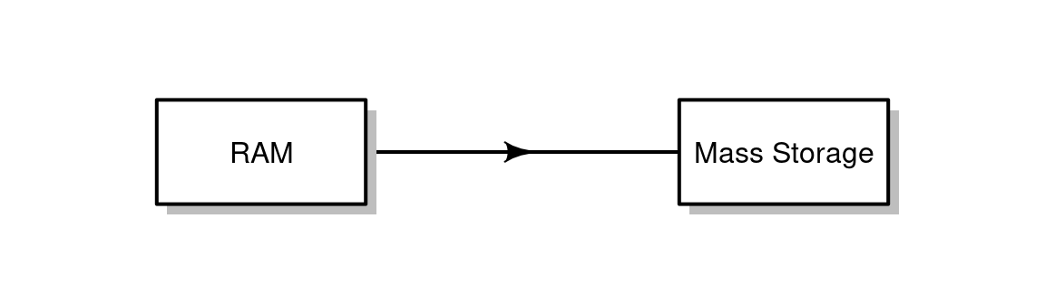
write.csv(dates, 'data/MOD13A3_2000_2019_dates2.csv', row.names = FALSE)

Figure 4.8: Writing data from the RAM to long-term storage.

Like in read.csv, we can either give a full file path or just the file name. If we specify just the file name, such as in the above example, the file is written to the working directory.

The additional row.names parameter determines whether the row names are saved. As mentioned above (Section 4.1.4), data.frame row names are usually meaningless, in which case there is no reason to save them in the CSV file. Therefore we typically use row.names=FALSE.

References

Murrell, Paul. 2009. Introduction to Data Technologies. CRC Press.

Wickham, Hadley et al. 2011. “The Split-Apply-Combine Strategy for Data Analysis.” Journal of Statistical Software 40 (1): 1–29.

R has other functions for reading tables in other formats, such as the read.xlsx function, from the openxlsx package, for reading Excel (.xlsx) files.↩︎
If there are numerous matches, the corresponding rows of x are duplicated to accomodate all matching values. This is usually an undesired situation. Therefore, we want to make sure that all values in the key column of y are unique, before doing a left join. That way, we make sure that no duplication takes place, and the join result contains exactly the same number of rows as x.↩︎
Population in 2019, based on Wikipedia.↩︎