2  Vector layers

2.1 Loading packages

First, we import three packages we will be working with:

• pandas—for working with tables,
• shapely—for working with individual geometries, and
• geopandas—for working with vector layers,

as follows:

import pandas as pd
import shapely
import geopandas as gpd

2.2 What is geopandas?

The geopandas package, an extension of the pandas package, is aimed at working with vector layers. To facilitate the representation of vector geometries and layers, geopandas defines two data structures, which are extensions of the analogous data structures from pandas for non-spatial data:

• GeoSeries—An extension of a Series for storing a sequence of geometries and a Coordinate Reference System (CRS) definition, where each geometry is a shapely object
• GeoDataFrame—An extension of a DataFrame, where one of the columns is a GeoSeries

As will be demostrated in a moment (see Section 2.3), a GeoDataFrame, representing a vector layer, is thus a combination (Figure 2.1) of:

• A GeoSeries, which holds the geometries in a special “geometry” column
• Zero or more Series, which represent the non-spatial attributes

Figure 2.1: GeoDataFrame structure (source: https://geopandas.org/getting_started/introduction.html)

The geopandas package depends on several other Python packages, most importantly:

• numpy
• pandas
• fiona—Interface to GDAL
• shapely—Interface to GEOS
• pyproj—Interface to PROJ

To put it another way, geopandas may be considered a high-level “wrapper” of fiona, shapely, and pyproj, giving access to all (or most) of their functionality through pandas-based data structures and a uniform interface.

2.3 Vector layer from scratch

2.3.1 Overview

In the first example, we create a vector layer from scratch. That way, we will be familiar with the hierarchical structure of the vector layer components:

• Separate geometries (shapely.geometry.*)
• Geometry column (GeoSeries)
• Vector layer (GeoDataFrame)

2.3.2 Separate geometries (shapely.geometry.*)

To create a geometry object (shapely.geometry.*, package shapely), we can pass a list of coordinates, or geometries, to the respective shapely.* function, according to the geometry type. The seven commonly used Simple Feature geometry types (Figure 2.2) are supported.

Figure 2.2: Simple feature geometry types

For example, here is how we create three POINT geometries, named pnt1, pnt2, and pnt3, using function shapely.Point:

pnt1 = shapely.Point([16.9418, 52.4643])
pnt2 = shapely.Point([16.9474, 52.4436])
pnt3 = shapely.Point([16.9308, 52.4437])

Note the type of the resulting objects:

type(pnt1)

shapely.geometry.point.Point

Printing a shapely geometry object in Jupyter Notebook draws a small figure:

pnt1

The print function prints the Well Known Text (WKT) representation of the geometry:

print(pnt1)

POINT (16.9418 52.4643)

2.3.3 Geometry column (GeoSeries)

To create a geometry column (GeoSeries, package geopandas), we pass a list of shapely geometries to the gpd.GeoSeries function. The second (optional) argument of gpd.GeoSeries is a crs, specifying the Coordinate Reference System (CRS). In this case, we specify the WGS84 geographical CRS, using its EPSG code 4326:

geom = gpd.GeoSeries([pnt1, pnt2, pnt3], crs=4326)
geom

0    POINT (16.94180 52.46430)
1    POINT (16.94740 52.44360)
2    POINT (16.93080 52.44370)
dtype: geometry

One of the first things we might want to do with a GeoSeries is to .plot it, to examine what it looks like (Figure 2.3):

geom.plot();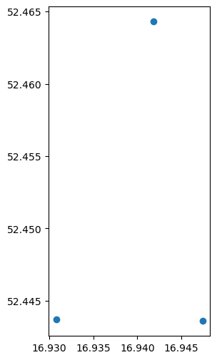

Figure 2.3: GeoSeries with three points of interest in Poznan

Besides the GeoSeries, a vector layer typically contains one or more Series, representing non-spatial columns (Figure 2.1), such as for numeric, text, or boolean data. For example, let’s create a Series called name, with the names of the point locations in geom, using pd.Series:

name = pd.Series([
    'Faculty of Geographical and Geological Sciences', 
    'Hotel ForZa', 
    'HL Hotel Lechicka'
])
name

0    Faculty of Geographical an...
1                      Hotel ForZa
2                HL Hotel Lechicka
dtype: object

2.3.4 Vector layer (GeoDataFrame)

A vector layer (GeoDataFrame, package geopandas) is a table with a geometry column (GeoSeries) along with zero or more “ordinary” columns (Series) (AKA “attributes”). Or, in other words, a vector layer is an extension of an ordinary table (DataFrame, package pandas), where one of the columns is a GeoSeries.

One way to create a GeoDataFrame is to pass a dict of Series and GeoSeries to the gpd.GeoDataFrame function. For example, here we combine name and geom into a GeoDataFrame named poi (“points of interest”):

poi = gpd.GeoDataFrame({'name': name, 'geometry': geom})
poi

	name	geometry
0	Faculty of Geographical an...	POINT (16.94180 52.46430)
1	Hotel ForZa	POINT (16.94740 52.44360)
2	HL Hotel Lechicka	POINT (16.93080 52.44370)

Figure 2.4 summarizes the above workflow of constructing a vector layer from scratch:

• Individual geometries—shapely objects (package shapely)
• Geometry column—GeoSeries objects
• Vector layer—GeoDataFrame object

Figure 2.4: Creating a GeoDataFrame from scratch

Figure 2.5 shows the hierarchical structure of GeoDataFrame, using another vector layer (two points, London and Paris):

• The entire vector layer is a GeoDataFrame object
• The geometric part, i.e., the geometry column, is a GeoSeries object
• Each cell in the geometry column, i.e., an individual geometry, is a shapely object (package shapely)

Figure 2.5: Structure of a GeoDataFrame

Note

For those familiar with R, Table 2.1 gives a summary of the analogous classes in R and Python for columns, tables, and vector layers.

Table 2.1: Classes in R and Python for columns, tables, and vector layers

Concept	R class {package}	Python class {package}
Column	numeric,character… {base}	Series {pandas}
Table	data.frame {base}	DataFrame {pandas}
Geometry	sfg {sf}	shapely.geometry.* {shapely}
Geometry column	sfc {sf}	GeoSeries {geopandas}
Vector layer	sf {sf}	GeoDataFrame {geopandas}

2.4 Reading from file

We can also import an existing vector layers from a file. In the next example, we import a Shapefile named gis_osm_transport_a_free_1.shp. This is a polygonal layer with the transport-related features around Poznan. The Shapefile is a processed subset of OpenStreetMap data, downloaded from geofabrik.

To import a vector layer from a file, we use the gpd.read_file function:

pol = gpd.read_file('data/osm/gis_osm_transport_a_free_1.shp')
pol

	osm_id	code	fclass	name	geometry
0	27923283	5656	apron	NaN	POLYGON ((16.84088 52.4247...
1	28396243	5656	apron	NaN	POLYGON ((16.96750 52.3274...
2	28396249	5656	apron	NaN	POLYGON ((16.98029 52.3239...
...	...	...	...	...	...
279	1101813658	5601	railway_station	NaN	POLYGON ((16.52227 52.3442...
280	1146503680	5641	taxi	NaN	POLYGON ((16.90591 52.4287...
281	1157127550	5641	taxi	NaN	POLYGON ((18.07060 51.7482...

282 rows × 5 columns

We can see that the geometry type, in this case, is POLYGON.

2.5 Subsetting by attributes

Subsetting a GeoDataFrame by attributes works the same way as for a DataFrame in pandas. We create a boolean Series, using conditions applied on one or more columns, then pass the Series as an index.

For example, here we subset the OSM transport-related polygons matching a specific 'name':

sel = 'Port Lotniczy Poznań-Ławica im. Henryka Wieniawskiego'
pol = pol[pol['name'] == sel]
pol

	osm_id	code	fclass	name	geometry
116	342024881	5651	airport	Port Lotniczy Poznań-Ławic...	POLYGON ((16.80040 52.4249...

2.6 Plotting 1

A GeoDataFrame also has a .plot method (Figure 2.6):

pol.plot();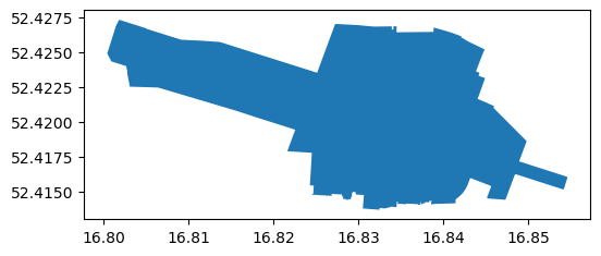

Figure 2.6: Plot of a GeoDataFrame with one POLYGON (Poznan airport)

Two of the most useful parameters of .plot (Figure 2.7) are:

• color—Polygon interior fill color (or point/line color)
• edgecolor—Polygon border color

pol.plot(color='none', edgecolor='black');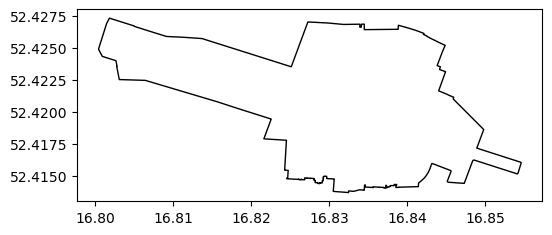

Figure 2.7: Setting color and edgecolor in .plot

2.7 Table to point layer

In the next example, we are going to read a text file representing public transport stations (with lon/lat), and convert it to a point layer. The file stops.txt contains the public transport stops in Poznan, downloaded from the GTFS repository for Poznan.

Even though the file extension is .txt, this is actually a CSV file. To read a CSV file, we can use the pd.read_csv function. The result is a DataFrame, where we also drop one of the irrelevant columns ('stop_code'):

stops = pd.read_csv('data/gtfs/stops.txt')
stops = stops.drop(columns='stop_code')
stops

	stop_id	stop_name	stop_lat	stop_lon	zone_id
0	2186	Żerniki/Skrzyżowanie	52.326840	17.042626	B
1	355	Sucholeska	52.462338	16.868885	A
2	4204	Pawłowicka	52.478103	16.786287	A
...	...	...	...	...	...
2918	3876	Witkowice/	52.497704	16.529493	C
2919	594	Międzyzdrojska	52.436424	16.808997	A
2920	1190	Koziegłowy/Zakłady Drobiar...	52.441243	16.998186	B

2921 rows × 5 columns

The columns named 'stop_lon' and 'stop_lat' contain the stop coordinates. The two columns, along with the CRS definition (4326 for lon/lat) can be transformed to a GeoSeries object, using the gpd.points_from_xy and the gpd.GeoSeries functions:

geom = gpd.points_from_xy(stops['stop_lon'], stops['stop_lat'], crs=4326)
geom = gpd.GeoSeries(geom)
geom

0       POINT (17.04263 52.32684)
1       POINT (16.86888 52.46234)
2       POINT (16.78629 52.47810)
                  ...            
2918    POINT (16.52949 52.49770)
2919    POINT (16.80900 52.43642)
2920    POINT (16.99819 52.44124)
Length: 2921, dtype: geometry

A GeoSeries can be combined with non-spatial attributes, to create a GeoDataFrame. Again, we use the gpd.GeoDataFrame function, but this time passing an existing DataFrame (data) and a GeoSeries (geometry):

stops = gpd.GeoDataFrame(data=stops, geometry=geom)
stops = stops.drop(columns=['stop_lon', 'stop_lat'])
stops

	stop_id	stop_name	zone_id	geometry
0	2186	Żerniki/Skrzyżowanie	B	POINT (17.04263 52.32684)
1	355	Sucholeska	A	POINT (16.86888 52.46234)
2	4204	Pawłowicka	A	POINT (16.78629 52.47810)
...	...	...	...	...
2918	3876	Witkowice/	C	POINT (16.52949 52.49770)
2919	594	Międzyzdrojska	A	POINT (16.80900 52.43642)
2920	1190	Koziegłowy/Zakłady Drobiar...	B	POINT (16.99819 52.44124)

2921 rows × 4 columns

2.8 Plotting 2

The resulting layer of stops is plotted below, using another argument of .plot (Figure 2.8):

• markersize—Point size

stops.plot(markersize=1);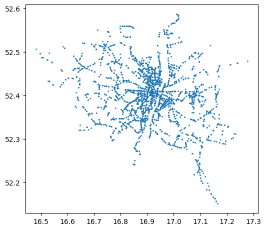

Figure 2.8: Setting markersize in .plot

A .plot with symbology can be created using the following parameters:

• column—A column name
• legend—Whether to show a legend
• cmap—Color map, such as from ColorBrewer and a wide variety of other options

For example, here we plot stops points colored according to their 'zone_id' (Figure 2.9):

stops.plot(markersize=1, column='zone_id', legend=True, cmap='Dark2');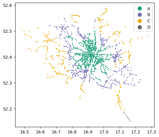

Figure 2.9: Setting symbology in .plot

To display more than one layer in the same plot, we need to:

• store the first plot in a variable (e.g., base), and
• pass it as the ax argument of any subsequent plot(s) (e.g., ax=base).

For example, here we plot stops and poi together (Figure 2.10):

base = stops.plot(markersize=0.1)
poi.plot(ax=base, color='red');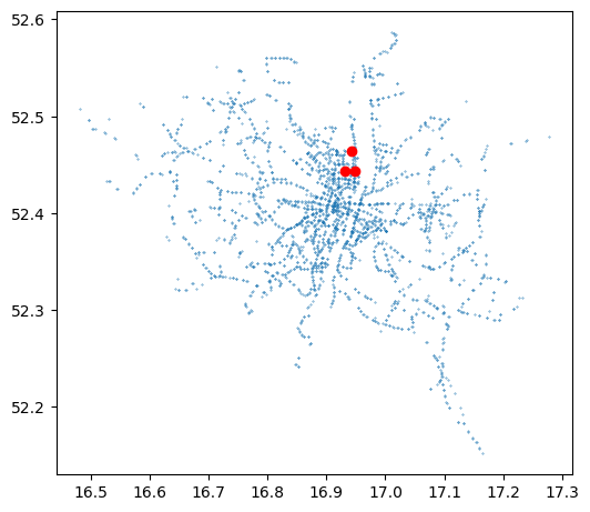

Figure 2.10: Displaying multiple layers in .plot

Another useful method to interactively examine the layer(s) is .explore. This creates an interactive map, with background for context:

stops.explore(column='zone_id', legend=True, cmap='Dark2')

Make this Notebook Trusted to load map: File -> Trust Notebook

For more information about mapping with geopandas, see the Mapping and Plotting Tools tutorial.

The next several examples demonstrate geoprocessing operations. geopandas provides the standard operators, using shapely and pyproj under the hood (which in turn are interfaces to the GEOS and PROJ software, respectively). For example:

• CRS and reprojection—Transforming a given layer from one CRS to another (Section 2.9)
• Numeric calculations—Calculating numeric geometry properties, such as length, area (Section 2.11), and distance
• New geometries—Creating new geometries, such as calculating buffers (Section 2.10), or area of intersection
• Geometric relations—Evaluating the relation between layers, such as whether two geometries intersect (Section 2.12)
• Spatial join—Joining attributes from one layer to another, based on spatial relations (Section 2.13)

2.9 Reprojection

An essential preliminary step in any spatial analysis that involves more than one layer is dealing with CRS. Typically, we must:

1. transform (reproject) all layers into the same CRS, so that they are aligned, and
2. make sure we use a projected CRS when making any distance- or area-related calculations

Important

All geometric calculations in geopandas (relying on shapely) assume planar geometry. Therefore, it only makes sense to calculate buffers, or areas, distance, etc., in projected CRS. Indeed, geopandas prints a warning otherwise. The spherely package, currently at an early stage of development, is aimed at filling this gap, based on Google’s s2 library for geometric calculations on the sphere (which R’s sf package already uses through package s2).

The existing Coordinate Reference System (CRS) definition of a GeoDataFrame (or a GeoSeries) is accessible through the .crs property. For example, here is the CRS information of the poi layer (WGS84, EPSG:4326):

poi.crs

<Geographic 2D CRS: EPSG:4326>
Name: WGS 84
Axis Info [ellipsoidal]:
- Lat[north]: Geodetic latitude (degree)
- Lon[east]: Geodetic longitude (degree)
Area of Use:
- name: World.
- bounds: (-180.0, -90.0, 180.0, 90.0)
Datum: World Geodetic System 1984 ensemble
- Ellipsoid: WGS 84
- Prime Meridian: Greenwich

Reprojecting a vector layer means re-calculating all of the layer coordinates, so that they are in agreement with the new CRS. This is done using the .to_crs method.

For example, here we reproject the poi layer to the UTM Zone 33N CRS (EPSG:32633):

poi = poi.to_crs(32633)
poi

	name	geometry
0	Faculty of Geographical an...	POINT (631915.601 5814453....
1	Hotel ForZa	POINT (632358.061 5812161....
2	HL Hotel Lechicka	POINT (631229.629 5812142....

Let’s do the same for the other two layers, pol and stops:

pol = pol.to_crs(32633)
stops = stops.to_crs(32633)

2.10 Buffers

The .buffer method calculates a buffer around each geometry in a GeoSeries, or a GeoDataFrame, according to the specified distance (in CRS units). It returns a GeoSeries with the resulting polygons. For example, here we create buffers of 150 \(m\) around each point in poi:

b = poi.buffer(150)
b

0    POLYGON ((632065.601 58144...
1    POLYGON ((632508.061 58121...
2    POLYGON ((631379.629 58121...
dtype: geometry

The result is a GeoSeries, plotted below (Figure 2.11):

base = poi.plot()
b.plot(ax=base, color='none', edgecolor='black');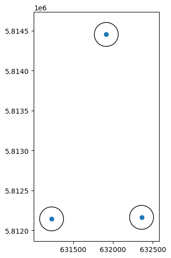

Figure 2.11: Buffers of three points calculated with .buffer

We often want to “keep” the attributes of the original geometries along with the new/derived geometries (such as buffers). To do that, we can assign the resulting GeoSeries as a secondary geometry column (we could also overwrite the original geometry column, in case we no longer need it):

poi['buffer_150'] = b
poi

	name	geometry	buffer_150
0	Faculty of Geographical an...	POINT (631915.601 5814453....	POLYGON ((632065.601 58144...
1	Hotel ForZa	POINT (632358.061 5812161....	POLYGON ((632508.061 58121...
2	HL Hotel Lechicka	POINT (631229.629 5812142....	POLYGON ((631379.629 58121...

We will also rename the original geometry column to point, to distinguish it from buffer_150:

poi = poi.rename(columns={'geometry': 'point'})
poi

	name	point	buffer_150
0	Faculty of Geographical an...	POINT (631915.601 5814453....	POLYGON ((632065.601 58144...
1	Hotel ForZa	POINT (632358.061 5812161....	POLYGON ((632508.061 58121...
2	HL Hotel Lechicka	POINT (631229.629 5812142....	POLYGON ((631379.629 58121...

Only one geometry column at a time is “active”, i.e., being accessed in geometrical calculations, plotting, etc. To switch the active geometry column, we can use the .set_geometry method:

poi = poi.set_geometry('buffer_150')
poi

	name	point	buffer_150
0	Faculty of Geographical an...	POINT (631915.601 5814453....	POLYGON ((632065.601 58144...
1	Hotel ForZa	POINT (632358.061 5812161....	POLYGON ((632508.061 58121...
2	HL Hotel Lechicka	POINT (631229.629 5812142....	POLYGON ((631379.629 58121...

The active geometry column, regardless of its name, can always be accessed through the .geometry property:

poi.geometry

0    POLYGON ((632065.601 58144...
1    POLYGON ((632508.061 58121...
2    POLYGON ((631379.629 58121...
Name: buffer_150, dtype: geometry

2.11 Area

As an example of a numeric calculation, the .area property gives the area sizes of the geometries, in CRS units (\(m^2\)).

For example, here are the areas of the (150-\(m\) buffer!) geometries in poi. Naturally, they are identical, and approximately equal to \(π\times150^2\):

poi.area

0    70572.341037
1    70572.341037
2    70572.341037
dtype: float64

As another example, here is the Poznan airport area is \(2,810,689\) \(m^2\):

pol.area

116    2.810689e+06
dtype: float64

2.12 Subsetting by location

Subsetting a vector layer by intersection with another vector layer can be done in three steps:

• Creating a shapely geometry representing the area of interest
• Evaluating intersection, using the .intersects method
• Subsetting using the resulting boolean Series

For example, to select stops that are within the poi buffers, we first create a “dissolved” individual geometry of all buffers, using .unary_union:

poi.unary_union

Next, we use the .intersects method to evaluate whether each stops geometry intersects with the buffers:

sel = stops.intersects(poi.unary_union)
sel

0       False
1       False
2       False
        ...  
2918    False
2919    False
2920    False
Length: 2921, dtype: bool

The resulting boolean Series named sel can be used to subset stops. The subset of stops is then assigned to a new layer, hereby named stops_in_b:

stops_in_b = stops[sel]
stops_in_b

	stop_id	stop_name	zone_id	geometry
295	418	UAM Wydział Geografii	A	POINT (631866.974 5814440....
681	467	Umultowska	A	POINT (631093.642 5812201....
1724	468	Umultowska	A	POINT (631203.588 5812071....
1861	417	UAM Wydział Geografii	A	POINT (631899.728 5814565....

Note

The above example demonstrate the “many to one” mode of .intersects, where the relation is evaluated between each of several geometries in a GeoSeries/GeoDataFrame, and an individual shapely geometry (Figure 2.12). Another mode, not shown here, is pairwise evaluation between two GeoSeries/GeoDataFrames.

Figure 2.12: “Many to one” mode of .intersects and analogous functions (source: https://geopandas.org/en/stable/docs/reference/api/geopandas.GeoSeries.intersects.html)

Note

There are methods analogous to .intersects for all other standard predicates, such as .contains, .touches, .within, etc.

Figure 2.13 shows the stops_in_b subset, along with the buffers used to create it:

base = stops_in_b.plot(color='red')
poi.set_geometry('point').plot(ax=base)
poi.plot(ax=base, color='none', edgecolor='black');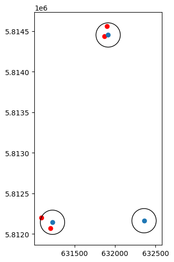

Figure 2.13: Three points of interest (in red), their buffers (in black), and bus stops that intersect with the buffers (in blue)

Here is an interactive view of the same result, also demonstrating how to show multiple layers with .explore:

m = poi.explore(color='black', style_kwds={'fill': False, 'weight': 3})
m = stops_in_b.explore(m=m, color='red', marker_kwds={'radius': 5})
poi.set_geometry('point').explore(m=m, marker_kwds={'radius': 5})

Make this Notebook Trusted to load map: File -> Trust Notebook

2.13 Spatial join

Spatial join attaches the attributes of the second layer y, to the first layer x, matched based on intersection (or another predicate) between the geometries. For example, a spatial join of the buffers (poi) and the bus stops (stops) means that the buffers will obtain the attributes of the stop(s) that are inside each buffer.

With geopandas, spatial join can be done using the .sjoin method. Namely, the expression x.sjoin(y) attaches the attributes of y to the matching features of x. Typically we are interested in a left join (how='left'), meaning that all features of x are retained, even if they match no geometries in y.

For example, the following expression attaches stops properties to each poi buffer:

poi.sjoin(stops, how='left')

	name	point	buffer_150	...	stop_id	stop_name	zone_id
0	Faculty of Geographical an...	POINT (631915.601 5814453....	POLYGON ((632065.601 58144...	...	418.0	UAM Wydział Geografii	A
0	Faculty of Geographical an...	POINT (631915.601 5814453....	POLYGON ((632065.601 58144...	...	417.0	UAM Wydział Geografii	A
1	Hotel ForZa	POINT (632358.061 5812161....	POLYGON ((632508.061 58121...	...	NaN	NaN	NaN
2	HL Hotel Lechicka	POINT (631229.629 5812142....	POLYGON ((631379.629 58121...	...	468.0	Umultowska	A
2	HL Hotel Lechicka	POINT (631229.629 5812142....	POLYGON ((631379.629 58121...	...	467.0	Umultowska	A

5 rows × 7 columns

In agreement with Figure 2.13, we can see that two of the buffers were joined with two bus stops (each), while one buffer (Hotel ForZa) had no matching bus stops at all.

2.14 Writing to file

To export a GeoDataFrame to a vector layer file, we use its .to_file method. The file format is automatically determined according to the chosen file extension, such as:

• .shp—Shapefile
• .gpkg—GeoPackage
• .geojson—GeoJSON

For example, here is how we can export the poi layer to a GeoPackage file named pol.gpkg. Note that we are dropping the secondary (point) geometry column before exporting:

poi.drop(columns='point').to_file('poi_buffer_150.gpkg')

Figure 2.14 shows the exported file when opened in QGIS.

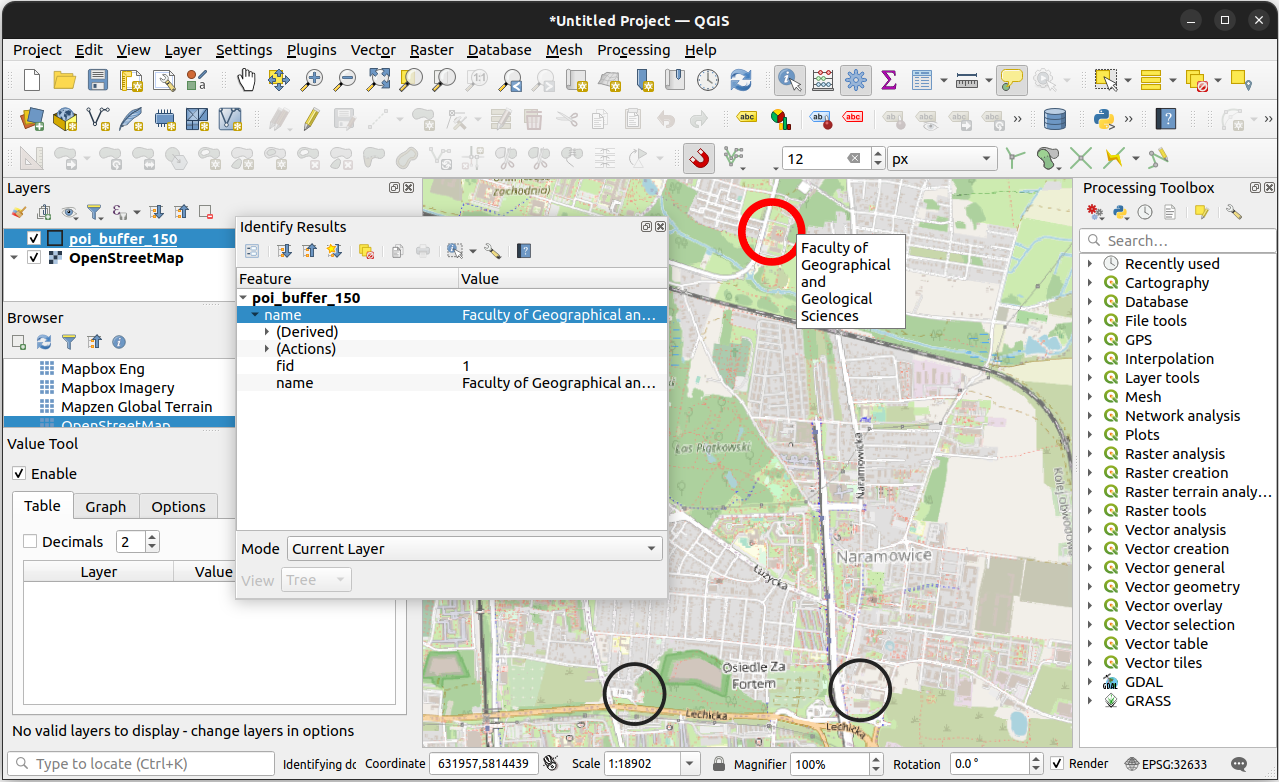
Figure 2.14: Exported vector layer file poi_buffer_150.gpkg viewed in QGIS

2.15 More information

See the Introduction to GeoPandas tutorial (Figure 2.15), and other sections in the geopandas documentation, for more information about geopandas.

Figure 2.15: The Introduction to GeoPandas tutorial