import pandas5 Python Setup
5.1 Summary
The following is a summary of setup instructions on Windows, also described in detail below.
Download and install Miniconda (see Section 5.4). This will install Python and the Anaconda package manager.
Open the “Anaconda Prompt” from the Start menu (see Section 5.5) as administrator, then type
conda install -c conda-forge notebookto install thenotebookPython package (see Section 5.7.2).Run the
conda installexpression two more times, replacingnotebookwithgeopandasand thenrasterio, to also install these two packages:conda install -c conda-forge geopandasconda install -c conda-forge rasterio
Open the Anaconda Prompt as a normal user, and type
jupyter notebook.Create a Notebook file (
.ipynb), or open an existing one, and start writing/running code (see Section 5.6)
Note
Other types of setup are possible. The important thing is to have a Python environment with Jupyter Notebook and the geopandas and rasterio packages installed. (If you are using software other than Miniconda, please make sure that the matplotlib, folium, and mapclassify packages are also installed; using the Miniconda instructions should install them automatically.)
Important
You can self-check whether your Python setup works fine by following Exercise 3 at the end of this document (Figure 5.10).
5.2 Introduction
In this document we cover the prerequisites to setup the Python environment and interface, before we start actually learning about Python code in the tutoral. As we will see, there are quite a few preliminary steps.
More specifically, before starting to write Python code you need to install and learn how to use several software components:
- Miniconda, which is a popular Python package manager, and includes the Python program itself (see Section 5.4 and Section 5.5)
- The Jupyter Notebook interface, which can be installed from within Miniconda (see Section 5.5.4 and Section 5.6) and is the de-facto standard editor for writing and executing Python code in the data science domain
- Several Python packages, most importantly
geopandasandrasterio(and their dependenciesnumpy,pandas, andshapely), which we are going to use in the tutorial and are essential to work with arrays, tables, vector layers and rasters (see Section 5.7), also installed from within Miniconda
We also cover the concept of file paths (see Section 5.8), which is essential for importing from files and exporting to files in your Python scripts.
5.3 Running Python code
5.3.1 Python setup
There are several types of working environments that facilitate writing and running Python code. The common feature of all those environments is that they communicate with the Python interpreter. However, each environment also has other features that facilitate writing code and viewing the results. Python working environments include:
- The Python command line (Section 5.5.2)
- IPython (Section 5.5.3)
- Jupyter Notebooks (Section 5.5.4)
The Python program itself, as well as the environments used to access it and manage its packages (Section 5.7), are bundled into various software packages. For example, Python can be downloaded and installed in a minimalist standalone program, or as part of a package management system, such as Anaconda or Miniconda (which we will use). Python is also commonly incorporated into other software installations, including GIS software such as QGIS, ArcGIS or ArcPro, where it can be accessed through an internal command line. (Finally, Mac OS and Linux typically come with a built-in “system” Python installation.)
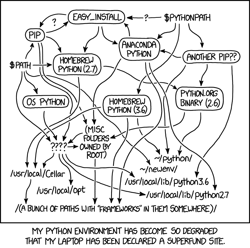
Python setup methods and environemnts are notoriously variable, whereas multiple Python versions on the same computer may conflict and “break” (Figure 5.1). In this chapter we aim to use one of the simplest and safest methods, based on Miniconda.
5.3.2 What software will we use?
The main component we are going to use is the Miniconda software. Miniconda is the recommended way to install Python on your computer for the purposes of the tutorial (and in general). Miniconda is the minimalist version of the well-known Anaconda software. Miniconda includes just Python, the conda package manager for Python (see Section 5.7.2), and few other packages, whereas Anaconda comes with over 250 pre-installed Python packages. However, the pre-installed packages in Anaconda do not include most spatial packages we are going to need.
All software components we need other than Miniconda, namely Jupyter Notebook and other Python packages, can be installed through the Miniconda command line. Therefore, a prerequisite to the following material is that you have Miniconda installed (see Section 5.4), that you have access to the Miniconda command prompt (Section 5.5), and that you can run Miniconda as administrator to install the required packages (see Section 5.7.2), or you have those packages already installed (e.g., by the IT administrator).
It is important to note that Python, Miniconda, and the third-party Python packages we are going to use in the tutorial are free and open-source. Therefore, you can flexibly use these tools later on, in any setting and at no cost: at work in a commercial company, in the academy, in personal projects at home, and so on.
The instructions in this chapter assume the Windows 10 operating system.
5.4 Installing Miniconda
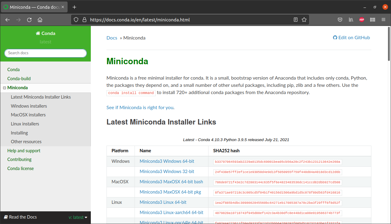
To install Miniconda, go to the Miniconda website (Figure 5.2), choose the right installation file for your system (such as Miniconda3 Windows 64-bit), download the file and execute it to run the installation process. Choose the default options when asked.
5.5 Using the miniconda command line
5.5.1 The Miniconda command line
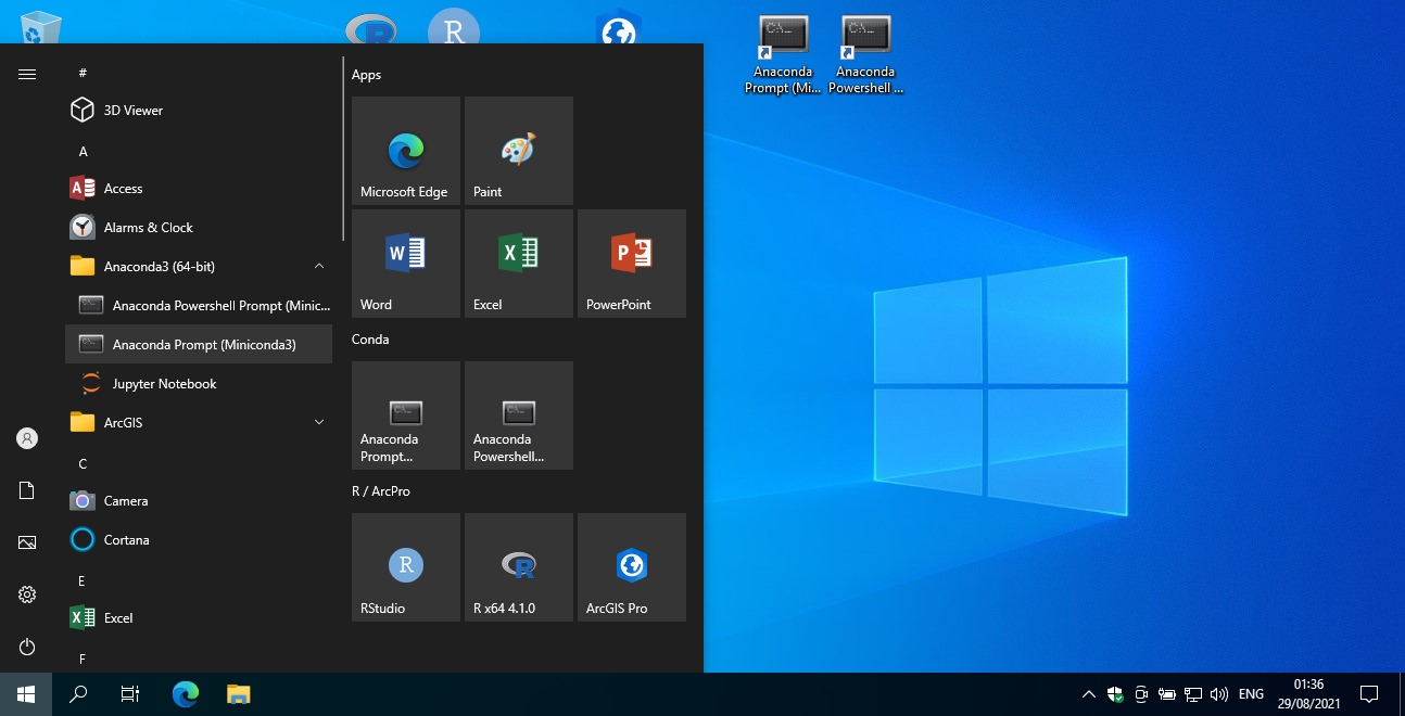
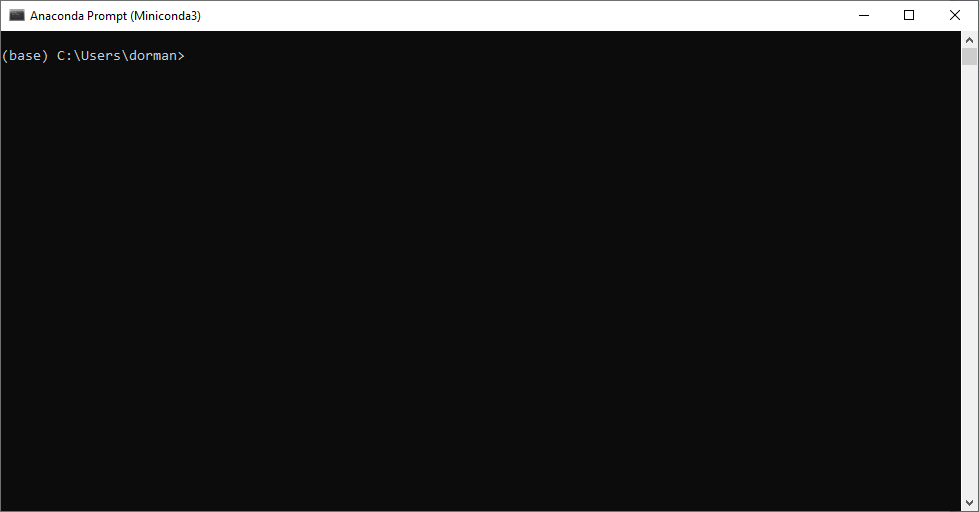
To start the miniconda command line, locate the Anaconda Prompt (Miniconda3) entry in your Start menu (Figure 5.3), and click on it.
You should see a command line window (Figure 5.4). Just like in any command-line interface, you can type and execute commands. For working with Python, in this tutorial and in general, you need to be familiar with just few commands:
- Commands to move through drives and directories:
cd—Short for “change directory”, to move through the directory structure (in the same drive), as incd C:\Users\dorman\DownloadsX:—To switch to a different drive, type the drive name followed by colon, as inD:to switch to driveD:\dir—To list current directory contents
- Commands to run programs:
python—Starting the Pyton command line interface (see Section 5.5.2)ipython—Starting the IPython interface (see Section 5.5.3)jupyter notebook—Starting the Jupyter Notebook interface (see Section 5.5.4)conda install—Installing third-party Python packages (see Section 5.7.2)
Miniconda can thus be thought of as an extended version of the ordinary computer’s command line (“cmd”), where the Python program (python) and Python package management tool (conda) are pre-installed.
You can exit from the Miniconda command line by closing the window, or by typing exit and pressing Enter.
Tip
A newer and more convenient command line is the Windows Terminal. It can be used as an alternative to the Anaconda Prompt. To use the Windows Terminal, you first need to install it, then associate it with the Anaconda Prompt through the settings.
5.5.2 The Python command line
The first and simplest thing that the Miniconda command line provides, is the basic command-line interface to Python, i.e., the python program. The Python command line can be accessed by typing python in the miniconda command line (see Section 5.5):
pythonThis opens the Python command line, which is marked by the >>> symbol.
Once inside the Python command line, Python expressions can be typed and executed by pressing Enter. For example, Figure 5.5 shows what it looks like to open the Python command line and execute the two expressions, which define a list object and print it:
a = [1,2,3]
print(a)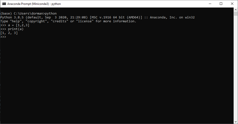
The Python command line is convenient for experimenting with short and simple commands. When our code gets bigger and more complex, we usually prefer to keep it in persistent code files so that we can keep a record of our code, using Python script files (.py), or Jupyter notebooks (.ipynb) (see Section 5.5.4).
To exit the Python command line, and return to the miniconda command line, type exit() and press Enter:
exit()5.5.3 IPython
IPython (“Interactive Python”) can be thought of as an enhanced Python command-line application, with many additional features. For example, IPython introduces new helper commands (such as ? for getting help), more sophisticated autocompletion, shortcuts for interacting with the operating system, and more. Importantly, working with IPython involves a series of cells, with code input (marked with In) and output (marked with Out).
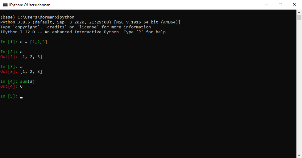
The IPython command line can be accessed by typing ipython in the miniconda command line (see Section 5.5):
ipythonYou can exit from IPython (and return to the Miniconda command line) by typing exit, or exit(), and pressing Enter:
exit5.5.4 Jupyter Notebook
Jupyter Notebook is an extended interface of IPython, where, on top of the interactive interpreter and formatting, we also have a web interface to edit “notebooks” that permanently contain both the code and the output. Additionally, notebooks may contain formatted text, tables, images, equations, etc. (Figure 5.7).

To use Jupyter Notebook, you need to install the notebook package, similarly to the way that any other Python package is installed. The notebook package includes the Jupyter Notebook interface program. For example, when using miniconda, the following expression can be used to install notebook:
conda install -c conda-forge notebookOpen the miniconda command line as administrator (by right-clicking on the miniconda command line icon, then choosing Run as administrator), then run the above command to install notebook. See Section 5.7.2 for more details and instructions to install notebook, and the other packages we will be working with in the tutorial. When done, go back to this section to experiment with the notebook interface.
To start the Jupyter Notebook interface, open the Miniconda command line again as an ordinary (non-administrator) user, and navigate to the directory where your notebooks are stored (or where you would like to create a new notebook). Then, run jupyter notebook to start the Jupyter Notebook interface:
jupyter notebookFor example, if your working directory is C:\Users\dorman\Downloads, then you need to start the miniconda command-line and run the following two expressions to open the Jupyter Notebook interface (for example, to create a new notebook):
cd C:\Users\dorman\Downloads
jupyter notebook
or the following expression to open an existing notebook named code_01.ipynb:
cd C:\Users\dorman\Downloads
jupyter notebook code_01.ipynb
Tip
cd, one of the most useful commands in the command line, stands for “change directory”. Another useful command is dir, which prints directory contents. Try it out!
After running jupyter notebook, you should see some output printed in the console (Figure 5.8). At the same time, the notebook interface should automatically open in the browser (Figure 5.7).
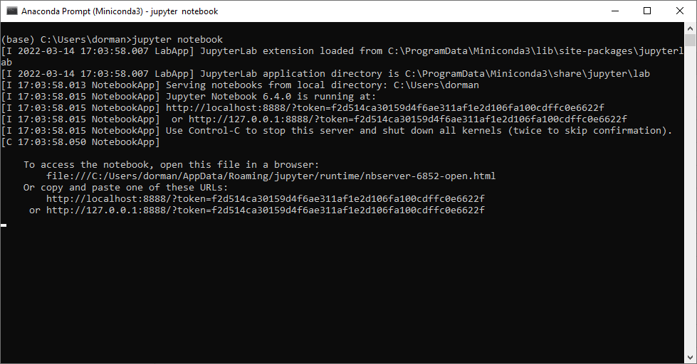
jupyter notebookJupyter notebooks are viewed and executed through a web browser, but they need to be connected to a running Python process. Therefore leave the console open as long as you are working with the Jupyter notebooks in the browser. When done, first close the Jupyter notebook tab(s) in the browser, and then terminate the jupyter notebook process with Ctrl+C.
Note
Jupyter Lab, which you can install with conda install -c conda-forge jupyterlab, is a newer and more sophisticated alternative to Jupyter Notebook with some additional features (such as a built-in command line). However, the basic functionality of editing and running .ipynb files are identical in Jupyter Notebook and Jupyter Lab, so you can use either one of them for the purposes of the tutoria.
5.6 Working with notebooks
5.6.1 Notebook files (.ipynb)
Notebooks are saved as .ipynb files (short for “IPython notebook”). .ipynb are plain text files, but more sophisticated ones then .py script files. Importantly, .ipynb files contains not just Python code inputs, but also:
- the division into separate “cells” (see Section 5.5.3),
- code outputs (see Section 5.6.5), both textual and graphical ones, resulting from previous evaluations of the code cells (see Section 5.6.4), if any, and
- non-code cells (see Section 5.6.2). (Do not worry if these terms are not clear yet—we are going to demonstrate them shortly.)
Accordingly, and unlike a plain .py script file, an .ipynb file does not make much sense when viewing and editing though an plain text editor. It is intended to be viewed and edited only through an interface that can process and display it, such as Jupyter Notebook.
A notebook documents the Python workflow, so that it can be kept for future reference or shared with other people.
To create a new notebook in the Jupyter Notebook interface:
- Click on the New button (in the top-right of the screen)
- Click on Python 3
This should open a new browser tab displaying the new notebook. By default, the notebook will be named Untitled.ipynb. You can rename it through File→Rename… in the menu (or clicking on the file name, in the top ribbon). While working with the notebook, and before closing it, remember to save your progress using the File→Save and Checkpoint, or by pressing Ctrl+S.
You can also open an existing notebook, by running jupyter notebook and then choosing it in the file browser, which displays all files in the directory where the jupyter notebook command was executed. Alternatively, you can open a partucular notebook directly from the command line by specifying its name. For example, to open the notebook named code_01.ipynb in the current working directory run jupyter notebook code_01.ipynb.
Exercise 1
- Open the Miniconda command line.
- Navigate to your working directory, using a command such as
cd C:\Users\dorman\Downloads. - Start the Jupyter Notebook interface, using the
jupyter notebookcommand. - Create a new Jupyter Notebook.
- Rename the notebook to any name other than the default, such as
code_01.ipynb. - Save the notebook.
- Close the browser tab, then stop the Jupyter Notebook interface using Ctrl+C in the Miniconda command line.
- Re-open the notebook you just created, using a command such as
jupyter notebook code_01.ipynb.
5.6.2 Cell types
Jupyter notebooks are composed of cells. There are two types of cells:
- Code cells
- Non-code cells, also known as Markdown cells
You can distinguish between code cells and non-code cells, by the In [...] part displayed to the left of code cells (Section 5.5.4).
Code cells contain Python code, which can be executed, displaying the result (if any) immediately below the cell. We elaborate on code execution (Section 5.6.4) and code output (Section 5.6.5) below.
Markdown cells contain text, typically explanations, or background information, describing the code. Markdown cells follow the Markdown syntax, so in addition to plain text they may display headings, bold or italic text, bullet lists, tables, URLs, and so on. For example, the online version of the book you are reading right now is prepared from a set of Jupyter notebooks (one for each chapter), where all contents other then code are set using Markdown syntax. You can download the source .ipynb files of the tutorial to see how various elements, such as bullet lists, tables, etc., are specified.
5.6.3 Working modes
There are two “modes” when working inside a notebook:
- Navigation mode
- Cell editing mode
You can switch between the two modes as follows:
- When in the navigation mode, you can enter editing mode by pressing Enter. That way, you can edit the current cell.
- To exit editing mode, and return to navigation mode, press Esc.
When in navigation mode, there are quite a few things, related to cell organization, that you can do. The most common operations are summarized in Table 5.1.
| Keyboard shortcut | Operation |
|---|---|
| ↑ / ↓ | Navigate between cells |
| A | Create new cell above current one |
| B | Create new cell below current one |
| D, D | Delete current cell |
| Y | Convert the current cell to a code cell |
| M | Convert the current cell to a markdown cell |
| C | “Copy” current cell |
| X | “Cut” current cell |
| V | “Paste” the copied or cut cell, below current cell |
When in editing mode, you can type or edit cell contents, much like in a plain text editor. If the cell is a code cell, then the text is interpreted as Python code. If the cell is a markdown cell, then the text is interpreted as markdown text.
5.6.4 Executing cells
You can execute a cell by pressing Ctrl+Enter, or Shift+Enter. The difference between the two is that the latter advances to the next cell (Table 5.2). These keyboard shortcuts work in both editing and navigation modes.
- When executing a code cell, the code is sent to the underlying Python interpreter, and the result (if any) is displayed below the cell.
- When executing a markdown cell, the text is rendered, so that any formatting (such as bold text marked with
**) is displayed
| Keyboard shortcut | Operation |
|---|---|
| Ctrl+Enter | Execute current cell |
| Shift+Enter | Execute current cell & advance |
Note that you can navigate between cells, skip cells, and execute the cells in a notebook, in any order you choose. The Python process in the background keeps track of the current state of the environment as a result of all code you have run so far. You can always reset the environment using the Kernel→Restart button in the menu. In general, it makes sense to write the notebook assuming the cells will be executed in the given order. To run the entire notebook, from start to finish, you can use the Kernel→Restart & Run All button.
Exercise 2
- Create a Jupyter notebook and try the operations described above, as follows.
- Create two or more code cells, and two or more markdown cells
- Type some code into the code cells, and execute it using Ctrl+Enter. We have not learned any Python syntax yet. For now, you can insert the code expressions shown above to create and type a list (see Section 5.5.2), or arithmetic expressions such as
10+5. - Type text into the markdown cells and “execute” them too to display the text. (You can also check out markdown syntax rules online and use them to format your text.)
- Delete one of the cells by pressing the D key twice.
5.6.5 Code output
Code output appears below a code cell, in case it has already been executed. It is important to understand that a Jupyter Notebook, in an .ipynb file, may store code as well as output. This is unlike a plain Python script, in a .py file, which stores just Python code, withouth any output. You can always remove all outputs from a notebook using the Kernel→Restart & Clear Output button. Alternatively, you can use the Kernel→Restart & Run All button to run the entire notebook from start to finish, thus calculating (or updating) all code outputs at once.
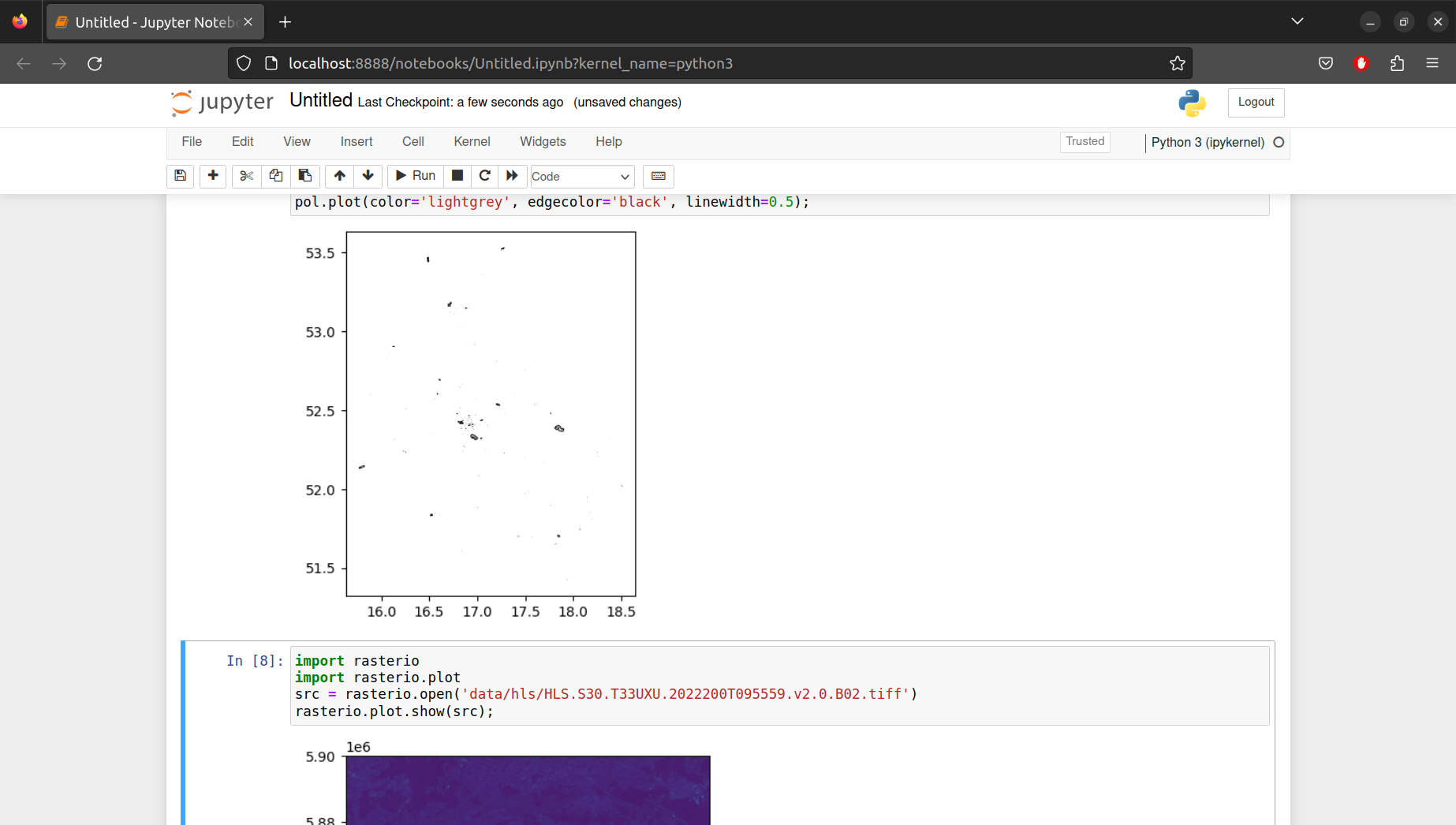
Usually, code output in a Jupyter notebook is just textual, in which case it is displayed in the notebook exactly the same way as it would appear in a Python command line (see Section 5.5.2), or in an IPython command line (see Section 5.5.3). However, since Jupyter notebooks are displayed in a web browser, they are able to dispay many other types of non-textual output that the command line cannot display. For example, Jupyter notebooks can display images such as plots or maps (Figure 5.10), which result from Python functions.
5.7 Python packages
5.7.1 What are packages?
Packages are code collections that we can import in our Python script, or a Jupyter notebook, to make the functions defined there available to us.
The Python installation comes with numerous built-in packages, known as Python’s standard library (https://docs.python.org/3/library/). For example, the csv package, which provides a basic method of reading CSV files, is part of the standard library. Packages from the standard library, such as csv, do not need to be installed. However, they need to be loaded before use (see Section 5.7.3).
There are many Python packages that are not part of the standard Python installation, known as third-party packages, or external packages. For example, pandas is a third-party Python package which has more advanced methods for reading CSV files than the csv package. Since third-party packages are not part of the Python installation, they need to be installed in a separate step (see Section 5.7.2). Once installed, third-party packages need to be loaded before use (see Section 5.7.3), just like standard packages.
5.7.2 Installing packages
When using Miniconda, Python packages can be installed from the Miniconda command line, using an expression such as:
conda install -c conda-forge PACKAGEwhere the word PACKAGE needs to be replaced with the package name. For example, here is the specific expression that can be used to install the geopandas package:
conda install -c conda-forge geopandasRemember that the Minoconda command line must be started as administrator when installing packages (see Section 5.5.4)!
To run the examples in this tutorial, you need to install several packages, most importantly geopandas and rasterio. Installing geopandas installs several dependencies that we mention in the tutorial, such as numpy, pandas and shapely. Another package that we need to install, to read Excel files, is openpyxl. Therefore, you need to run three commands, one after the other, to install all required packages:
conda install -c conda-forge notebook
conda install -c conda-forge geopandas
conda install -c conda-forge rasterio
As part of the installation of each package, you will see a printout of the package dependencies and versions that are going to be installed. Type y (yes) and press Enter to approve and proceed with the installation (Figure 5.9). (The installation progress may take a few minutes; you may need top press Enter if you see that the process is stuck.)
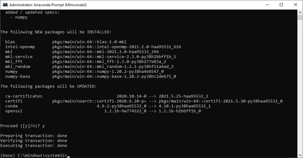
conda install on the miniconda command line
Tip
To keep things simple, the above instructions in fact describe “manual” installation of packages in the default (base) environment of Anaconda. The generally recommended approach, which you should adopt when working with Python, is, however:
- to install (specific versions of) all required packages at once, based on a file listing them (e.g.,
.yml), - in a separate “environment” for each project.
To create an environment in Anaconda according to a .yml file listing the required packages, use the command conda env create -f environment.yml. For example, you can download the environment.yml file, which lists the required packages for this tutorial. This will create an environment named tutorial (as specified in this particular environment.yml file) and install specific versions of the required packages with (again, as specified in the environment.yml file).
Once the tutorial environment was created, you can “activate” it using conda activate tutorial. This will display (tutorial) instead of (base) at the beginning of the command line. Practically, this means that the Python installation is “switched” to work with a separate directory of installed packages. Once inside the environment, all of the other instructions in the tutorial apply: you can navigate to the required directory, open the Jupyter Notebook interface with jupyter notebook (since the notebook package was already installed, as it was listed in environment.yml), etc. When done, you can “deactivate” the environment (going back to base) using the command deactivate.
Tip
Installation of packages with conda can be quite slow. A faster alternative is mamba. To use it, first install mamba with conda install mamba -n base -c conda-forge, then use it to install other packages, as in mamba install -c conda-forge geopandas.
5.7.3 Loading packages
A package can be loaded using the import keyword, followed by package name. For example, here is how we can import the pandas package (for working with tables in Python):
Afterwards, we can access any function from the package, by typing pandas.*. For example, here we create a Series (labelled 1-dimensional array) object:
pandas.Series([1, 3, 5])0 1
1 3
2 5
dtype: int64It is common practice to import a package under a different name which is shorter to type, using the import package as name expression. For example, by convention the pandas package is usually imported under the name pd:
import pandas as pdWe can now access all of the functions in pandas using pd.*, instead of pandas.*:
pd.Series([1, 3, 5])0 1
1 3
2 5
dtype: int645.8 File paths
Simple Python scripts may be self-contained, in the sense that the data they operate on are created as part of the script itself, and the results are not saved to permanent strage (e.g., on the hard disk). However, in realistic data analysis it is often necessary to:
- import existing data from disk at the beginning of the script, and to
- export the results to a file on disk at the end.
For example, here is a short script that reads a Shapefile and plots the contained vector layer:
import geopandas as gpd
pol = gpd.read_file('data/osm/gis_osm_transport_a_free_1.shp')
pol.plot(color='lightgrey', edgecolor='black', linewidth=0.5);
Do not worry about the functions and methods used in the code, as we are going to cover them in the tutorial. For now, pay attention just to the the file path "data/osm/gis_osm_transport_a_free_1.shp".
First, note that, in Python code, unlike in the Miniconda command line (see {ref}using-miniconda-command-line), you must use /, and not \ when writing file paths!
Second, note that data/osm/gis_osm_transport_a_free_1.shp is a relative path, in which we specify a partial path that begins with the notebook location. For example, the relative path "data/osm/gis_osm_transport_a_free_1.shp", means that we refer to:
- the file named
osm/gis_osm_transport_a_free_1.shp, - which is located in the
osmdirectory, - which is located in the
datadirectory, - which is located in the directory where our notebook or script is.
Specifying the just a file name, such as "gis_osm_transport_a_free_1.shp" is a special case of a relative path, meaning that the file is located in the same directory where our script is.
In all other code examples in the tutorial, we are going to use relative file paths starting with data, such as "data/osm/gis_osm_transport_a_free_1.shp". To reproduce the examples, therefore, you need to:
- download source tutorial.zip archive, which includes
.ipynbJupyter notebooks and thedatadirectory with sample data files, - extract the files from the archive,
- open the notebook files
vector.ipynb(Chapter 2) orraster.ipynb(Chapter 3) in the Jupyter Notebook interface (see Section 5.5.4), and - run the code
Exercise 3
- Download tutorial.zip and extract the files. This results in the file structure shown below:
- Open the Anaconda Prompt (Miniconda3) program
- Navigate to the
tutorialdirectory with the extracted files, using a command such asdir cd C:\Users\dorman\Downloads\tutorial - Run the command
jupyter notebookto open the Jupyter Notebook interface - Create a new notebook
- Create a new cell with the following code section, which uses the
geopandaspackage to read and plot a vector layer:
import geopandas as gpd
pol = gpd.read_file('data/osm/gis_osm_transport_a_free_1.shp')
pol.plot(color='lightgrey', edgecolor='black', linewidth=0.5);- Create another cell which uses the
rasteriopackage to read and plot a raster:
import rasterio
import rasterio.plot
src = rasterio.open('data/hls/HLS.S30.T33UXU.2022200T095559.v2.0.B02.tiff');
rasterio.plot.show(src)- Execute the cells
- If all worked well, you should see a plot with polygons (Figure 5.10)