import glob
import matplotlib.pyplot as plt
import numpy as np
import geopandas as gpd
import rasterio
import rasterio.plot
import rasterio.mask3 Rasters
3.1 Loading packages
First, we import several packages we will be working with:
glob—for listing file paths,matplotlib.pyplot—for plotting a raster layer and a vector layer together,numpy—for working with arrays,geopandas—for working with vector layers, andrasterio,rasterio.plot,rasterio.mask—for working with rasters,
as follows:
3.2 What is rasterio?
Working with rasters in Python is not as well-organized around one dominant and comprehensive package, such as geopandas for vector layers. Instead, there are several packages providing alternative (subsets of) methods for working with rasters, and each of them may require working with further helper or extension packages for specific tasks.
rasterio—which we use in this tutorial—is a well-established and widely-used Python package for working with rasters. rasterio makes raster data accessible in the form of numpy arrays associated with a “metadata” object, so that we can operate on them, then write back to new raster files. rasterio, like most raster processing software, is based on the GDAL software. Compared to geopandas (Chapter 2), the rasterio package will seem more “low-level”. And, as mentioned above, it needs to be complemented with other packages for specific tasks, such the rasterstats package for zonal statistics.
Alternatively, each of the packages rioxarray, xarray-spatial, and geowombat, were developed as “high-level” alternatives to rasterio, using an xarray-based representation of rasters (compared to rasterio, which is numpy-based). These packages are higher-level, representing rasters in a single object with both data and metadata. They are, therefore, easier to work with, but less well-established than rasterio (and similarly not feature-complete).
3.3 Reading from file
The rasterio package works with the concept of a file connection, a pointer to a file on disk, with associated methods for reading from or writing to. A rasterio file connection to a raster file has two components:
- The metadata (such as the dimensions, resolution, CRS, etc.)
- A reference to the raster values (Figure 3.1)
The raster values are thus not immediately read into memory. Instead, whenever necessary, the values can be read, either all at once, or from a particular band, or from a “window”, or at a particular resolution. The rationale is that the metadata are small (and often useful to examine on their own), while values are often very big. Therefore, it can be more practical to have control over which values to read, and when.

rasterio) structureTo create a file connection object to a raster file, we use the rasterio.open function. For example, here we create a file connection object named src, which refers to the HLS.S30.T33UXU.2022200T095559.v2.0.B02.tiff raster:
src = rasterio.open('data/hls/HLS.S30.T33UXU.2022200T095559.v2.0.B02.tiff')
src
<open DatasetReader name='data/hls/HLS.S30.T33UXU.2022200T095559.v2.0.B02.tiff' mode='r'>This file is:
- one of the four sample data files (
B02=blue band, see Section 3.5), - comprising a Landsat-8 and Sentinel-2 satellite-image based reflectance raster,
- from the Harmonized Landsat Sentinel-2 (HLS) Surface Reflecance product, which provides global observations of the land every 2–3 days at 30-\(m\) spatial resolution,
- from
2022-07-19, - tile ID
T33UXU(covering Poznan), - downloaded from EarthData Search.
Note that the file connection specifies mode='r', i.e., reading mode, which is the default of rasterio.open. When writing a raster file, we create a file connection (possibly to a not yet existing file) in writing mode (mode='w') (Section 3.5).
The raster metadata can be accessed through the .meta property of the file connection. For example, from the following metadata object:
src.meta{'driver': 'GTiff',
'dtype': 'int16',
'nodata': -9999.0,
'width': 3660,
'height': 3660,
'count': 1,
'crs': CRS.from_epsg(32633),
'transform': Affine(30.0, 0.0, 600000.0,
0.0, -30.0, 5900040.0)}we can learn that:
- Raster file format (
driver) is GeoTIFF - Raster data type (
dtype) is 16-bit integer (int16), i.e.,-32768to32767 - The value representing “No Data” (
nodata) is-9999 - Raster size (
width,height) is \(3,660\times3,660\) pixels - The number of bands (
count) is \(1\) - Raster CRS (
crs) is UTM Zone 33N (EPSG code32633) - Raster origin and resolution (
transform) are (600000.0,5900040.0) and (30,30), respectively
The raster values can be read using the .read method. The default is to read all values (as mentioned above, there are many other options to read partial data):
r = src.read()
r
array([[[427, 440, 430, ..., 209, 328, 362],
[449, 412, 439, ..., 315, 200, 233],
[415, 364, 388, ..., 399, 306, 231],
...,
[364, 393, 464, ..., 212, 280, 313],
[164, 174, 173, ..., 236, 260, 265],
[145, 143, 147, ..., 283, 286, 281]]], dtype=int16)The resulting object r is an ndarray object (package numpy):
type(r)numpy.ndarrayNote that array dimensions correspond to (bands,rows,columns), in that order. In our case, r has 1 band, 3660 rows, and 3660 columns:
r.shape(1, 3660, 3660)The array stores the values using the same data type as the original file:
r.dtypedtype('int16')This means that the minimal amount of RAM is being used, which is an advantage of rasterio over other Python packages (e.g., rioxarray which imports all rasters as float), and programming languages such as R.
3.4 Plotting (single-band)
The rasterio.plot.show function (from the rasterio.plot “sub-package”) can be used to plot a raster. This function can accept a file connection (see below), or an array (see Section 3.12).
For example, the following expression plots the raster from the src file connection, using reversed greyscale ('Greys_r') colormap:
rasterio.plot.show(src, cmap='Greys_r');
3.5 Stacking raster bands
Remote sensing products, such as satellite images, are often distributed as a collection of single-band files, one file for each spectral band of the sensor. As specified in the HLS product description, the file we just read (B02) represents blue reflectance. Overall, the following files are included in the sample data:
B02—BlueB03—GreenB04—RedB08—Near Infra Red (NIR)
In this section we will stack the four separate files into one multi-band raster file. As we will see, this involves reading the files in a for loop, and writing each band into a raster file connection created in writing mode.
Using the standard Python package glob, here is how we can obtain a list of all file paths matching a particular pattern:
files = glob.glob('data/hls/*.tiff')
files
['data/hls/HLS.S30.T33UXU.2022200T095559.v2.0.B08.tiff',
'data/hls/HLS.S30.T33UXU.2022200T095559.v2.0.B02.tiff',
'data/hls/HLS.S30.T33UXU.2022200T095559.v2.0.B04.tiff',
'data/hls/HLS.S30.T33UXU.2022200T095559.v2.0.B03.tiff']Typically satellite bands are ordered according to wavelength, from shortest (in our case, Blue) to longest (in our case, NIR). Since the latter matches alphabetical order, we can sort using the .sort method, as follows:
files.sort()
files
['data/hls/HLS.S30.T33UXU.2022200T095559.v2.0.B02.tiff',
'data/hls/HLS.S30.T33UXU.2022200T095559.v2.0.B03.tiff',
'data/hls/HLS.S30.T33UXU.2022200T095559.v2.0.B04.tiff',
'data/hls/HLS.S30.T33UXU.2022200T095559.v2.0.B08.tiff']Writing rasters with rasterio can be thought of as the reverse of reading (Figure 3.1). Namely, we need to pass a metadata object when creating a file connection, and then write array(s) of values into the file connection.
To read the data from files, and write them into a new multi-band file, using rasterio, our strategy is as follows:
- Creating a metadata object for the new file
- Creating a file connection to a (non-existing) file with the given metadata in
'w'mode - For each file in
files:- Reading the data into an
ndarray - Writing the data into the corresponding band in the new file
- Reading the data into an
- Closing the file connection
The metadata for the multi-band file is identical to the single-band metadata, with the exception of the count property (number of bands). Therefore, we don’t need to create the metadata from scratch. Instead, we re-use the existing metadata object:
meta = src.meta
meta
{'driver': 'GTiff',
'dtype': 'int16',
'nodata': -9999.0,
'width': 3660,
'height': 3660,
'count': 1,
'crs': CRS.from_epsg(32633),
'transform': Affine(30.0, 0.0, 600000.0,
0.0, -30.0, 5900040.0)}while modifying band count according to the number of files:
meta.update(count=len(files))
meta
{'driver': 'GTiff',
'dtype': 'int16',
'nodata': -9999.0,
'width': 3660,
'height': 3660,
'count': 4,
'crs': CRS.from_epsg(32633),
'transform': Affine(30.0, 0.0, 600000.0,
0.0, -30.0, 5900040.0)}Now that we have the metadata object, we create a “destination” file connection, hereby named dst, in writing mode 'w'. The new file is named hls.tif:
dst = rasterio.open('hls.tif', 'w', **meta)
dst
<open DatasetWriter name='hls.tif' mode='w'>Next, we iterate over the files, each time reading the current band and writing it to the destination file:
for index, filename in enumerate(files, start=1):
    src = rasterio.open(filename)
    dst.write(src.read(1), index)
    src.close()
Finally, we close the file connection, to make sure that all data have been written:
dst.close()Now, we create a file connection src to the newly created file to keep working with it. Examining the metadata shows that indeed it has four bands ('count':4):
src = rasterio.open('hls.tif')
src.meta
{'driver': 'GTiff',
'dtype': 'int16',
'nodata': -9999.0,
'width': 3660,
'height': 3660,
'count': 4,
'crs': CRS.from_epsg(32633),
'transform': Affine(30.0, 0.0, 600000.0,
0.0, -30.0, 5900040.0)}Using .read we can read the data from all (four) bands, as follows:
r = src.read()
r
array([[[ 427, 440, 430, ..., 209, 328, 362],
[ 449, 412, 439, ..., 315, 200, 233],
[ 415, 364, 388, ..., 399, 306, 231],
...,
[ 364, 393, 464, ..., 212, 280, 313],
[ 164, 174, 173, ..., 236, 260, 265],
[ 145, 143, 147, ..., 283, 286, 281]],
[[ 743, 765, 790, ..., 420, 607, 678],
[ 740, 716, 770, ..., 556, 372, 444],
[ 672, 620, 685, ..., 713, 575, 423],
...,
[ 795, 872, 983, ..., 522, 571, 633],
[ 420, 444, 440, ..., 545, 593, 640],
[ 424, 415, 412, ..., 734, 746, 727]],
[[1118, 1183, 1221, ..., 364, 634, 709],
[1068, 1048, 1175, ..., 529, 274, 354],
[ 932, 881, 1004, ..., 698, 470, 310],
...,
[ 512, 564, 652, ..., 342, 497, 576],
[ 283, 293, 278, ..., 366, 398, 413],
[ 226, 229, 239, ..., 465, 445, 457]],
[[1985, 2003, 2106, ..., 2732, 2479, 2376],
[1827, 1791, 2035, ..., 3052, 3144, 2980],
[1629, 1566, 1797, ..., 2875, 3333, 3492],
...,
[4365, 4482, 4576, ..., 3464, 3004, 2961],
[4082, 4007, 4103, ..., 3461, 3564, 3656],
[4328, 4499, 4674, ..., 3670, 3730, 3489]]], dtype=int16)r is now a three-dimensional ndarray with four bands:
r.shape(4, 3660, 3660)When opened in QGIS, with bands 3-2-1 mapped to Red-Green-Blue, the hls.tif raster appears as shown in Figure 3.3.
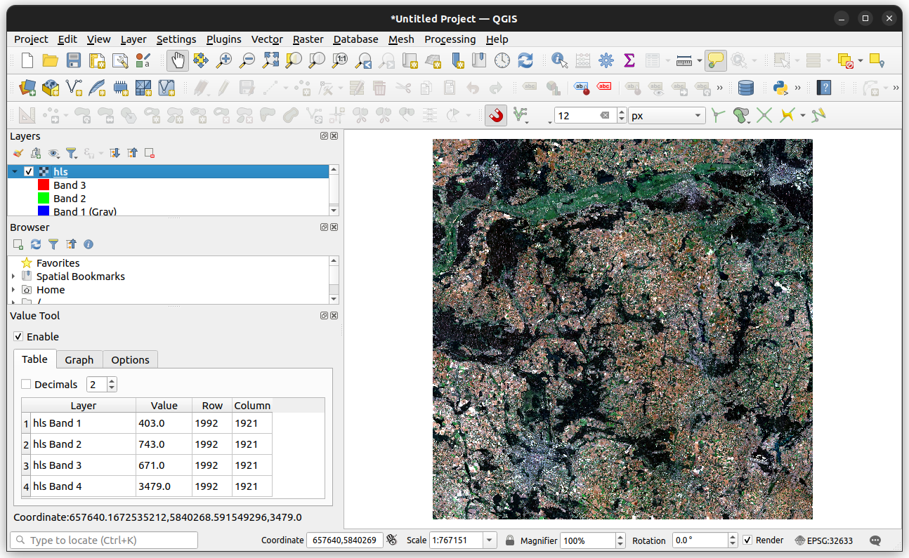
hls.tif viewed in QGIS3.6 Data types
As shown above, numpy arrays are also associated with specific data types (all array values are of the same type). These correspond to raster file data types. Commonly used data types in numpy are summarized in Table 3.1. As you can see, there are many varieties of numeric types in numpy. This may seem confusing, compared to basic Python or other programming languages such as R, which have just one data type for integer and one for float. However, keep in mind that the purpose of having many specific data types is conserving memory and making calculations more efficient.
| Data type | Description |
|---|---|
bool_ |
Boolean (True or False) stored as a byte |
int_ |
Platform-dependent default integer type (normally int64 or int32) |
int8 |
Integer in a single byte (-128 to 127) |
int16 |
Integer in 16 bits (-32768 to 32767) |
int32 |
Integer in 32 bits (-2147483648 to 2147483647) |
int64 |
Integer in 64 bits (-9223372036854775808 to 9223372036854775807) |
uint8 |
Unsigned integer (0 to 255) |
uint16 |
Unsigned integer (0 to 65535) |
uint32 |
Unsigned integer (0 to 4294967295) |
uint64 |
Unsigned integer (0 to 18446744073709551615) |
float_ |
Default float type, shorthand for float64 |
float16 |
Half-precision (16 bit) float (-65504 to 65504) |
float32 |
Single-precision (32 bit) float (1e-38 to 1e38) |
float64 |
Double-precision (64 bit) float (1e-308 to 1e308) |
For example, the HLS image we are working with is stored in the int16 data type. Accordingly, when reading the data into RAM, the resulting array is of type int16:
r.dtypedtype('int16')According to the product user guide, the HLS raster values:
- need to be rescaled by a factor of
0.0001, and - contain
-9999values representing “No Data”.
Rescaling is common practice in remote sensing product packaging. The rationale of rescaling is:
- The raster is stored in files using
intdata types, which takes less memory - It’s up to the user to rescale the values back to the valid range in “real” units, whenever they need to, which requires switching to
floatrepresentation, thus consuming more memory
“No Data” representation is important for int rasters, since (due to computer memory constraints, and unlike float rasters) int rasters cannot contain “native” “No Data” values. Instead, a specific integer value (e.g., -9999) is used as a “No Data” flag:
src.nodata-9999.0When reading an int raster into memory, again, it is up to the user to choose how to deal with the specific “No Data” flag. Ignoring it, however, will lead to wrong results, where the “No Data” pixels are treated as valid raster values:
r[r == src.nodata] ## i.e., r[r == -9999]array([-9999, -9999, -9999, -9999, -9999, -9999, -9999, -9999, -9999,
-9999, -9999, -9999, -9999, -9999, -9999, -9999], dtype=int16)Note that, technically, we’ve just used “boolean array indexing”, where a boolean array is used to subset a given array.
3.7 Changing the data type
Going back to the 4-band HLS reflectance raster, in practice, the following pre-processing steps are required:
- transforming
rto afloatdata type (this section), - replacing the value
-9999with the native “No Data” value (np.nan) (Section 3.8) - rescaling all values by a factor of
0.0001(Section 3.9) - truncating values which are beyond the valid range (Section 3.10)
To transform an ndarray to a different data type, we use the .astype method. The recommended approach is to use the platform-standard float data type, specified as np.float_ (Table 3.1), or simply float, typically resolving to np.float64:
r = r.astype(np.float_)
r
array([[[ 427., 440., 430., ..., 209., 328., 362.],
[ 449., 412., 439., ..., 315., 200., 233.],
[ 415., 364., 388., ..., 399., 306., 231.],
...,
[ 364., 393., 464., ..., 212., 280., 313.],
[ 164., 174., 173., ..., 236., 260., 265.],
[ 145., 143., 147., ..., 283., 286., 281.]],
[[ 743., 765., 790., ..., 420., 607., 678.],
[ 740., 716., 770., ..., 556., 372., 444.],
[ 672., 620., 685., ..., 713., 575., 423.],
...,
[ 795., 872., 983., ..., 522., 571., 633.],
[ 420., 444., 440., ..., 545., 593., 640.],
[ 424., 415., 412., ..., 734., 746., 727.]],
[[1118., 1183., 1221., ..., 364., 634., 709.],
[1068., 1048., 1175., ..., 529., 274., 354.],
[ 932., 881., 1004., ..., 698., 470., 310.],
...,
[ 512., 564., 652., ..., 342., 497., 576.],
[ 283., 293., 278., ..., 366., 398., 413.],
[ 226., 229., 239., ..., 465., 445., 457.]],
[[1985., 2003., 2106., ..., 2732., 2479., 2376.],
[1827., 1791., 2035., ..., 3052., 3144., 2980.],
[1629., 1566., 1797., ..., 2875., 3333., 3492.],
...,
[4365., 4482., 4576., ..., 3464., 3004., 2961.],
[4082., 4007., 4103., ..., 3461., 3564., 3656.],
[4328., 4499., 4674., ..., 3670., 3730., 3489.]]])We can use .dtype to see that, indeed, the data type has changed to np.float64:
r.dtypedtype('float64')3.8 Reclassify
Next, we replace the value -9999 with the native np.nan value (which is possible now that the array is of type float). This ensures that all subsequent arithmetic calculations, such as raster algebra (Section 3.9), actually “ignore” invalid pixels:
r[r == src.nodata] = np.nan
r
array([[[ 427., 440., 430., ..., 209., 328., 362.],
[ 449., 412., 439., ..., 315., 200., 233.],
[ 415., 364., 388., ..., 399., 306., 231.],
...,
[ 364., 393., 464., ..., 212., 280., 313.],
[ 164., 174., 173., ..., 236., 260., 265.],
[ 145., 143., 147., ..., 283., 286., 281.]],
[[ 743., 765., 790., ..., 420., 607., 678.],
[ 740., 716., 770., ..., 556., 372., 444.],
[ 672., 620., 685., ..., 713., 575., 423.],
...,
[ 795., 872., 983., ..., 522., 571., 633.],
[ 420., 444., 440., ..., 545., 593., 640.],
[ 424., 415., 412., ..., 734., 746., 727.]],
[[1118., 1183., 1221., ..., 364., 634., 709.],
[1068., 1048., 1175., ..., 529., 274., 354.],
[ 932., 881., 1004., ..., 698., 470., 310.],
...,
[ 512., 564., 652., ..., 342., 497., 576.],
[ 283., 293., 278., ..., 366., 398., 413.],
[ 226., 229., 239., ..., 465., 445., 457.]],
[[1985., 2003., 2106., ..., 2732., 2479., 2376.],
[1827., 1791., 2035., ..., 3052., 3144., 2980.],
[1629., 1566., 1797., ..., 2875., 3333., 3492.],
...,
[4365., 4482., 4576., ..., 3464., 3004., 2961.],
[4082., 4007., 4103., ..., 3461., 3564., 3656.],
[4328., 4499., 4674., ..., 3670., 3730., 3489.]]])This is an example of reclassifying raster values, where we convert all pixel values in a given range to a uniform value. Technically, this is another example of “boolean array indexing” (Section 3.7), only that we’ve also assigned a new value into the subset.
Here we demonstrate that the array no longer contains -9999 values:
r[r == src.nodata]array([], dtype=float64)3.9 Raster algebra
The next pre-processing step is rescaling. Array rescaling is an example of a “vectorized” operation, automatically carried out element-by-element on all array values, at once. In numpy terminology, this is known as “universal functions”.
For example, the following expression multiplies all values of array r by the scaling factor of 0.0001:
r = r * 0.0001
r
array([[[0.0427, 0.044 , 0.043 , ..., 0.0209, 0.0328, 0.0362],
[0.0449, 0.0412, 0.0439, ..., 0.0315, 0.02 , 0.0233],
[0.0415, 0.0364, 0.0388, ..., 0.0399, 0.0306, 0.0231],
...,
[0.0364, 0.0393, 0.0464, ..., 0.0212, 0.028 , 0.0313],
[0.0164, 0.0174, 0.0173, ..., 0.0236, 0.026 , 0.0265],
[0.0145, 0.0143, 0.0147, ..., 0.0283, 0.0286, 0.0281]],
[[0.0743, 0.0765, 0.079 , ..., 0.042 , 0.0607, 0.0678],
[0.074 , 0.0716, 0.077 , ..., 0.0556, 0.0372, 0.0444],
[0.0672, 0.062 , 0.0685, ..., 0.0713, 0.0575, 0.0423],
...,
[0.0795, 0.0872, 0.0983, ..., 0.0522, 0.0571, 0.0633],
[0.042 , 0.0444, 0.044 , ..., 0.0545, 0.0593, 0.064 ],
[0.0424, 0.0415, 0.0412, ..., 0.0734, 0.0746, 0.0727]],
[[0.1118, 0.1183, 0.1221, ..., 0.0364, 0.0634, 0.0709],
[0.1068, 0.1048, 0.1175, ..., 0.0529, 0.0274, 0.0354],
[0.0932, 0.0881, 0.1004, ..., 0.0698, 0.047 , 0.031 ],
...,
[0.0512, 0.0564, 0.0652, ..., 0.0342, 0.0497, 0.0576],
[0.0283, 0.0293, 0.0278, ..., 0.0366, 0.0398, 0.0413],
[0.0226, 0.0229, 0.0239, ..., 0.0465, 0.0445, 0.0457]],
[[0.1985, 0.2003, 0.2106, ..., 0.2732, 0.2479, 0.2376],
[0.1827, 0.1791, 0.2035, ..., 0.3052, 0.3144, 0.298 ],
[0.1629, 0.1566, 0.1797, ..., 0.2875, 0.3333, 0.3492],
...,
[0.4365, 0.4482, 0.4576, ..., 0.3464, 0.3004, 0.2961],
[0.4082, 0.4007, 0.4103, ..., 0.3461, 0.3564, 0.3656],
[0.4328, 0.4499, 0.4674, ..., 0.367 , 0.373 , 0.3489]]])3.10 Truncating to valid range
Since reflectance values are proportional, the valid range is between 0 (zero reflectance, i.e., completely dark) to 1 (complete reflectance, i.e., completely bright). Due to specific image acquisition and processing issues, the actual values may be beyond the valid range, in which case we may want to truncate them.
In our example, indeed the range of values in r goes beyong 0–1. We can use the np.nanmin and np.nanmax to obtain the minimum and maximum values in an array, respectively, excluding np.nan:
np.nanmin(r), np.nanmax(r)(-0.0339, 1.1088)Again, we can use “boolean array indexing” to “truncate” array values according to the valid range:
r[r < 0] = 0
r[r > 1] = 1
r
array([[[0.0427, 0.044 , 0.043 , ..., 0.0209, 0.0328, 0.0362],
[0.0449, 0.0412, 0.0439, ..., 0.0315, 0.02 , 0.0233],
[0.0415, 0.0364, 0.0388, ..., 0.0399, 0.0306, 0.0231],
...,
[0.0364, 0.0393, 0.0464, ..., 0.0212, 0.028 , 0.0313],
[0.0164, 0.0174, 0.0173, ..., 0.0236, 0.026 , 0.0265],
[0.0145, 0.0143, 0.0147, ..., 0.0283, 0.0286, 0.0281]],
[[0.0743, 0.0765, 0.079 , ..., 0.042 , 0.0607, 0.0678],
[0.074 , 0.0716, 0.077 , ..., 0.0556, 0.0372, 0.0444],
[0.0672, 0.062 , 0.0685, ..., 0.0713, 0.0575, 0.0423],
...,
[0.0795, 0.0872, 0.0983, ..., 0.0522, 0.0571, 0.0633],
[0.042 , 0.0444, 0.044 , ..., 0.0545, 0.0593, 0.064 ],
[0.0424, 0.0415, 0.0412, ..., 0.0734, 0.0746, 0.0727]],
[[0.1118, 0.1183, 0.1221, ..., 0.0364, 0.0634, 0.0709],
[0.1068, 0.1048, 0.1175, ..., 0.0529, 0.0274, 0.0354],
[0.0932, 0.0881, 0.1004, ..., 0.0698, 0.047 , 0.031 ],
...,
[0.0512, 0.0564, 0.0652, ..., 0.0342, 0.0497, 0.0576],
[0.0283, 0.0293, 0.0278, ..., 0.0366, 0.0398, 0.0413],
[0.0226, 0.0229, 0.0239, ..., 0.0465, 0.0445, 0.0457]],
[[0.1985, 0.2003, 0.2106, ..., 0.2732, 0.2479, 0.2376],
[0.1827, 0.1791, 0.2035, ..., 0.3052, 0.3144, 0.298 ],
[0.1629, 0.1566, 0.1797, ..., 0.2875, 0.3333, 0.3492],
...,
[0.4365, 0.4482, 0.4576, ..., 0.3464, 0.3004, 0.2961],
[0.4082, 0.4007, 0.4103, ..., 0.3461, 0.3564, 0.3656],
[0.4328, 0.4499, 0.4674, ..., 0.367 , 0.373 , 0.3489]]])Here we demonstrate that the range is now between 0 and 1:
np.nanmin(r), np.nanmax(r)(0.0, 1.0)3.11 Subsetting w/ indices
We can get a subset of array values using numeric indices, using an expression such as r[bands,rows,columns]. Each of the indices can be:
- an individual numeric value, e.g.,
0for the 1st element, or - a
list, e.g.,[0,2]for 1st and 3rd elements, or - a slice, e.g.,
0:3, or:3, for 1st (inclusive) through 4th (exclusive) elements.
The : symbol implies all elements.
For example, here is how we can subset r bands 1-3, all rows and all columns:
r[:3, :, :]array([[[0.0427, 0.044 , 0.043 , ..., 0.0209, 0.0328, 0.0362],
[0.0449, 0.0412, 0.0439, ..., 0.0315, 0.02 , 0.0233],
[0.0415, 0.0364, 0.0388, ..., 0.0399, 0.0306, 0.0231],
...,
[0.0364, 0.0393, 0.0464, ..., 0.0212, 0.028 , 0.0313],
[0.0164, 0.0174, 0.0173, ..., 0.0236, 0.026 , 0.0265],
[0.0145, 0.0143, 0.0147, ..., 0.0283, 0.0286, 0.0281]],
[[0.0743, 0.0765, 0.079 , ..., 0.042 , 0.0607, 0.0678],
[0.074 , 0.0716, 0.077 , ..., 0.0556, 0.0372, 0.0444],
[0.0672, 0.062 , 0.0685, ..., 0.0713, 0.0575, 0.0423],
...,
[0.0795, 0.0872, 0.0983, ..., 0.0522, 0.0571, 0.0633],
[0.042 , 0.0444, 0.044 , ..., 0.0545, 0.0593, 0.064 ],
[0.0424, 0.0415, 0.0412, ..., 0.0734, 0.0746, 0.0727]],
[[0.1118, 0.1183, 0.1221, ..., 0.0364, 0.0634, 0.0709],
[0.1068, 0.1048, 0.1175, ..., 0.0529, 0.0274, 0.0354],
[0.0932, 0.0881, 0.1004, ..., 0.0698, 0.047 , 0.031 ],
...,
[0.0512, 0.0564, 0.0652, ..., 0.0342, 0.0497, 0.0576],
[0.0283, 0.0293, 0.0278, ..., 0.0366, 0.0398, 0.0413],
[0.0226, 0.0229, 0.0239, ..., 0.0465, 0.0445, 0.0457]]])r[:3, :, :].shape(3, 3660, 3660)The last : indices can be omitted, therefore this gives the same result:
r[:3].shape(3, 3660, 3660)3.12 Plotting (RGB)
The rasterio.plot.show function automatically assumes that the first three bands refer to RGB, with range 0-255 (for int) or 0-1 (for float). Otherwise, we can rescale the values and/or rearrange the bands.
In our example, raster values are float and in the 0-1 range (as expected). However, the bands in reverse order than expected (BGR). To reverse the order of bands we can use the ::-1 slice:
r[:3][::-1]array([[[0.1118, 0.1183, 0.1221, ..., 0.0364, 0.0634, 0.0709],
[0.1068, 0.1048, 0.1175, ..., 0.0529, 0.0274, 0.0354],
[0.0932, 0.0881, 0.1004, ..., 0.0698, 0.047 , 0.031 ],
...,
[0.0512, 0.0564, 0.0652, ..., 0.0342, 0.0497, 0.0576],
[0.0283, 0.0293, 0.0278, ..., 0.0366, 0.0398, 0.0413],
[0.0226, 0.0229, 0.0239, ..., 0.0465, 0.0445, 0.0457]],
[[0.0743, 0.0765, 0.079 , ..., 0.042 , 0.0607, 0.0678],
[0.074 , 0.0716, 0.077 , ..., 0.0556, 0.0372, 0.0444],
[0.0672, 0.062 , 0.0685, ..., 0.0713, 0.0575, 0.0423],
...,
[0.0795, 0.0872, 0.0983, ..., 0.0522, 0.0571, 0.0633],
[0.042 , 0.0444, 0.044 , ..., 0.0545, 0.0593, 0.064 ],
[0.0424, 0.0415, 0.0412, ..., 0.0734, 0.0746, 0.0727]],
[[0.0427, 0.044 , 0.043 , ..., 0.0209, 0.0328, 0.0362],
[0.0449, 0.0412, 0.0439, ..., 0.0315, 0.02 , 0.0233],
[0.0415, 0.0364, 0.0388, ..., 0.0399, 0.0306, 0.0231],
...,
[0.0364, 0.0393, 0.0464, ..., 0.0212, 0.028 , 0.0313],
[0.0164, 0.0174, 0.0173, ..., 0.0236, 0.026 , 0.0265],
[0.0145, 0.0143, 0.0147, ..., 0.0283, 0.0286, 0.0281]]])We can also multiply the array by 4 to make the image brighter. Therefore (Figure 3.4):
rasterio.plot.show(r[:3][::-1]*4);Clipping input data to the valid range for imshow with RGB data ([0..1] for floats or [0..255] for integers).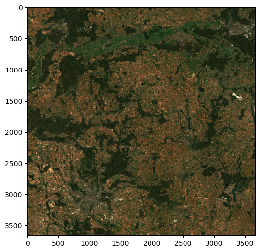
When plotting a standalone array, axes breaks reflect indices—since rasterio.plot.show has no knowledge of array the georeferencing. To show coordinates (as in plots of raster file connections, see Section 3.4), we can pass the transform matrix (Figure 3.5):
rasterio.plot.show(r[:3][::-1]*4, transform=src.transform);Clipping input data to the valid range for imshow with RGB data ([0..1] for floats or [0..255] for integers).![]()
3.13 Masking and cropping
Masking a raster means “erasing” values outside an area of interest, defined by polygon(s), by turning them into “No Data”. Cropping means that, additionally, we “shrink” the raster extent to eliminate empty rows and columns from the margins of the original extent.
In the following example, we are going to crop and mask the HLS image according the the bounding box of the Poznan airport buffered by 1 \(km\).
First, let’s re-create the airport polygon pol (Section 2.5):
pol = gpd.read_file('data/osm/gis_osm_transport_a_free_1.shp')
sel = 'Port Lotniczy Poznań-Ławica im. Henryka Wieniawskiego'
pol = pol[pol['name'] == sel]
pol = pol.to_crs(src.crs)
pol| osm_id | code | fclass | name | geometry | |
|---|---|---|---|---|---|
| 116 | 342024881 | 5651 | airport | Port Lotniczy Poznań-Ławica im. Henryka Wienia... | POLYGON ((622419.265 5809827.499, 622431.793 5... |
Next, we use the .buffer (Section 2.10) method to create a buffer of 1 \(km\). We then take the bounding box of the buffer using the .envelope property:
bbox = pol.buffer(1000).envelope
bbox
116 POLYGON ((621419.373 5807636.677, 627127.920 5...
dtype: geometryHere is an intractive view of the pol and bbox geometries:
m = bbox.explore()
pol.explore(m=m, color='red')
Make this Notebook Trusted to load map: File -> Trust Notebook
The rasterio.mask.mask function can be used for masking (and possibly cropping). It accepts the following arguments:
dataset—A raster file connection (e.g.,src)shapes—A list ofshapelypolygons (e.g.,bbox.to_list())crop—Whether to also reduce (i.e., crop) the raster extent according to the extent ofshapesnodata—Value to use for “No Data”. Typically:- a specific value (e.g.,
-9999) forintrasters, or np.nanforfloatrasters.
- a specific value (e.g.,
For example, here is how we can mask and crop the HLS image according to the bbox polygon(s):
out_image, out_transform = rasterio.mask.mask(
    src,
    bbox.to_list(),
    crop=True,
    nodata=-9999
)
Note that rasterio.mask.mask returns a tuple, which we immediately “unpack” into two variables, out_image:
out_imagearray([[[-9999, 479, 532, ..., 301, 285, -9999],
[-9999, 296, 220, ..., 379, 290, -9999],
[-9999, 836, 244, ..., 355, 276, -9999],
...,
[-9999, 342, 531, ..., 242, 330, -9999],
[-9999, 247, 458, ..., 414, 313, -9999],
[-9999, -9999, -9999, ..., -9999, -9999, -9999]],
[[-9999, 746, 848, ..., 492, 445, -9999],
[-9999, 591, 477, ..., 594, 507, -9999],
[-9999, 1162, 508, ..., 553, 535, -9999],
...,
[-9999, 626, 820, ..., 440, 555, -9999],
[-9999, 553, 756, ..., 684, 575, -9999],
[-9999, -9999, -9999, ..., -9999, -9999, -9999]],
[[-9999, 830, 918, ..., 366, 296, -9999],
[-9999, 577, 469, ..., 561, 351, -9999],
[-9999, 1295, 519, ..., 564, 331, -9999],
...,
[-9999, 848, 924, ..., 426, 580, -9999],
[-9999, 576, 840, ..., 744, 584, -9999],
[-9999, -9999, -9999, ..., -9999, -9999, -9999]],
[[-9999, 1952, 2158, ..., 2274, 2547, -9999],
[-9999, 2266, 2167, ..., 2633, 2806, -9999],
[-9999, 1956, 2297, ..., 2368, 3519, -9999],
...,
[-9999, 2444, 2212, ..., 2061, 2156, -9999],
[-9999, 2562, 2465, ..., 2246, 2102, -9999],
[-9999, -9999, -9999, ..., -9999, -9999, -9999]]], dtype=int16)and out_transform:
out_transformAffine(30.0, 0.0, 621390.0,
0.0, -30.0, 5811120.0)Since masking operates on the file connection, while all further processing steps were done in-memory, they need to be repeated on out_image:
out_image = out_image.astype(float)
out_image[out_image == -9999] = np.nan
out_image = out_image * 0.0001
out_image[out_image < 0] = 0
out_image[out_image > 1] = 1
The processed cropped array looks as follows:
out_imagearray([[[ nan, 0.0479, 0.0532, ..., 0.0301, 0.0285, nan],
[ nan, 0.0296, 0.022 , ..., 0.0379, 0.029 , nan],
[ nan, 0.0836, 0.0244, ..., 0.0355, 0.0276, nan],
...,
[ nan, 0.0342, 0.0531, ..., 0.0242, 0.033 , nan],
[ nan, 0.0247, 0.0458, ..., 0.0414, 0.0313, nan],
[ nan, nan, nan, ..., nan, nan, nan]],
[[ nan, 0.0746, 0.0848, ..., 0.0492, 0.0445, nan],
[ nan, 0.0591, 0.0477, ..., 0.0594, 0.0507, nan],
[ nan, 0.1162, 0.0508, ..., 0.0553, 0.0535, nan],
...,
[ nan, 0.0626, 0.082 , ..., 0.044 , 0.0555, nan],
[ nan, 0.0553, 0.0756, ..., 0.0684, 0.0575, nan],
[ nan, nan, nan, ..., nan, nan, nan]],
[[ nan, 0.083 , 0.0918, ..., 0.0366, 0.0296, nan],
[ nan, 0.0577, 0.0469, ..., 0.0561, 0.0351, nan],
[ nan, 0.1295, 0.0519, ..., 0.0564, 0.0331, nan],
...,
[ nan, 0.0848, 0.0924, ..., 0.0426, 0.058 , nan],
[ nan, 0.0576, 0.084 , ..., 0.0744, 0.0584, nan],
[ nan, nan, nan, ..., nan, nan, nan]],
[[ nan, 0.1952, 0.2158, ..., 0.2274, 0.2547, nan],
[ nan, 0.2266, 0.2167, ..., 0.2633, 0.2806, nan],
[ nan, 0.1956, 0.2297, ..., 0.2368, 0.3519, nan],
...,
[ nan, 0.2444, 0.2212, ..., 0.2061, 0.2156, nan],
[ nan, 0.2562, 0.2465, ..., 0.2246, 0.2102, nan],
[ nan, nan, nan, ..., nan, nan, nan]]])Note that the dimensions are now smaller:
out_image.shape(4, 117, 192)Here is a plot of the cropped image and the airport boundary (which is also an example of displaying a vector layer on top of a raster):
fig, ax = plt.subplots()
rasterio.plot.show(out_image[0:3][::-1]*4, transform=out_transform, ax=ax)
pol.plot(ax=ax, edgecolor='yellow', linewidth=0.5, color='none');
Clipping input data to the valid range for imshow with RGB data ([0..1] for floats or [0..255] for integers).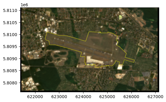
If necessary, here is how we can export the airport raster to a file named airport.tif:
meta.update(dtype=out_image.dtype)
meta.update(transform=out_transform)
meta.update(width=out_image.shape[2])
meta.update(height=out_image.shape[1])
dst = rasterio.open('airport.tif', 'w', **meta)
dst.write(out_image)
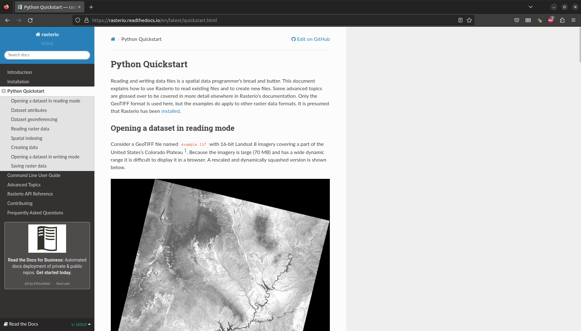
dst.close()3.14 More information
See the Python Quickstart tutorial (Figure 3.7), and other sections in the rasterio documentation, for more information about rasterio.