Chapter 6 Leaflet

6.1 Introduction

Now that we have covered the basics of web technologies, we are moving on to the main topic of this book: web mapping. This chapter and the next two (Chapters 6–8) introduce Leaflet, a JavaScript library used to create interactive web maps. Using Leaflet, you can create a simple map using just two or three JavaScript expressions, or you can build a complex map using hundreds of lines of code.

In this chapter, we will learn how to initialize a Leaflet web map on our web page, and how to add several types of layers on the map: tile layers (Section 6.5.7) and simple shapes such as point markers (Section 6.6.2), lines (Section 6.6.3), and polygons (Section 6.6.4). We will also learn to add interactive popups for our layers (Section 6.7) and a panel with a textual description of our map (Section 6.8). Finally, we will introduce map events—browser events associated with the web map (Section 6.9).

In the next two Chapters 7–8, we will learn some more advanced Leaflet functionality. In Chapter 7, we will learn to add complex shapes coming from external GeoJSON files. Then, in Chapter 8, we will learn how to define symbology and interactive behavior in our web map.

6.2 What is a web map?

We already introduced the concept of web mapping in Section 0.1. We mentioned that the term “web map” usually implies a map that is not simply on the web, but rather one that is powered by the web. It is usually interactive, and not always self-contained, meaning that it “pulls” content from other locations, such as tile layer servers (Section 6.5.8) or database APIs (Section 9.7)⁴⁶.

Similarly to spatial information displayed in GIS software, web maps are usually composed of one or more layers. Web map layers can be generally classified into two categories:

• Background layers, or basemaps, comprising collections of gridded images or vector tiles, which are usually general-purpose and not prepared specifically for our map
• Foreground layers, or overlays, which are usually vector layers (points, lines, and polygons), commonly prepared and/or fine-tuned for the specific map web where they are shown

Background layers are usually static and non-interactive. Conversely, foreground layers are usually dynamic and associated with user interaction, such as the ability to query layer attributes by clicking on a feature (Section 6.7).

6.3 What is Leaflet?

Leaflet (Crickard III 2014) is an open-source JavaScript library for building interactive web maps. Leaflet was initially released in 2011 (Table 6.1). It is lightweight, relatively simple, and flexible. For these reasons, Leaflet is probably the most popular open-source web-mapping library at the moment. As the Leaflet home page puts it, the guiding principle behind this library is simplicity:

“Leaflet doesn’t try to do everything for everyone. Instead it focuses on making the basic things work perfectly.”

Advanced functionality is still available through Leaflet plugins. Towards the end of the book, we will learn about two Leaflet plugins: Leaflet.heat (Section 12.6) and Leaflet.draw (Section 13.3).

6.4 Alternatives to Leaflet

In this book, we will exclusively use Leaflet for building web maps. However, it is important to be aware of the landscape of alternative web-mapping libraries, their advantages and disadvantages. Table 6.1 lists Leaflet along with other popular JavaScript libraries for web mapping⁴⁷.

TABLE 6.1: Popular web-mapping libraries

Library	Released	Type	URL
Google Maps	2005	Commercial	https://developers.google.com/maps/
OpenLayers	2006	Open-source	https://openlayers.org/
ArcGIS API for JS	2008	Commercial	https://developers.arcgis.com/javascript/
Leaflet	2011	Open-source	https://leafletjs.com/
D3	2011	Open-source	https://d3js.org/
Mapbox GL JS	2015	Commercial	https://www.mapbox.com/mapbox-gl-js/api/

Google Maps JavaScript API (Dincer and Uraz 2013) is a proprietary web-mapping library by Google. The biggest advantage of the Google Maps API is that it brings the finely crafted look and feel of the Google Maps background layer to your own web map. On the other hand, background layers other than Google’s are not supported. The Google Maps API also has advanced functionality not available elsewhere, such as integration with Street View scenes. However the library is closed-source, which means the web maps cannot be fully customized. Also, it requires a paid subscription.

OpenLayers (Gratier, Spencer, and Hazzard 2015; Langley and Perez 2016; Farkas 2016) is an older, more mature, and more richly featured open-source JavaScript library for building web maps, otherwise very similar to Leaflet in its scope. However, OpenLayers is also more complex, heavier (in terms of JavaScript file size), and more difficult to learn. Leaflet can be viewed as a lighter and more focused alternative to OpenLayers.

ArcGIS API for JavaScript (Rubalcava 2015) is another commercial web-mapping solution. The ArcGIS API is primarily designed to be used with services published using ArcGIS Online or ArcGIS Server, though general data sources can also be used. The ability of the ArcGIS API to tap into web services originating from ArcToolbox that perform geoprocessing on the server is a feature which has no good equivalent in open-source software. However, using an ArcGIS Server requires a paid (expensive) license. Also, the APIs are free to use for development or educational use, but require a fee for commercial use.

D3 (Murray 2017) is an open-source JavaScript library for visualization in general, though it is commonly used for mapping too (Newton and Villarreal 2014). D3 is primarily used for displaying vector layers, as raster tile layers are not well supported. D3 is probably the most complex and difficult to learn among the libraries listed in Table 6.1. However, it is very flexible and can be used to create truly innovative map designs. Go back to the examples from Section 0.1—some of the most impressive ones, such as Earth Weather, were created with the help of D3.

Mapbox GL JS is a web-mapping library provided by a commercial company named Mapbox. Notably, Mapbox GL JS uses customizable vector tile layers (Section 6.5.6.3) as background. You can use existing basemaps, or build your own using an interactive “studio” web application. Like Google Maps, Mapbox GL JS also requires a paid subscription, though the first 50,000 monthly map views are free.

6.5 Creating a basic web map

6.5.1 Overview

In this section, we will learn to create a basic web map using Leaflet. The map is going to contain a single background (tile) layer, initially zoomed-in on the Ben-Gurion University. The final result is shown in Figure 6.5.

6.5.2 Web page setup

We start with the following minimal HTML document, which we are familiar with from Chapter 1:

<!DOCTYPE html>
<html>
<head>
    <title>Basic map</title>
    <!-- More content will go here -->
</head>
<body>
    <!-- More content will go here -->
</body>
</html>

• Create an empty text file named index.html and copy the above code into that file.
• Follow the steps described in the Sections 6.5–6.8, to build your own web map from the ground up.

At this stage, the web page is empty. From here, we will do the following four things to add a map to our page:

• Include the Leaflet CSS file using a <link> element and the Leaflet JavaScript file using a <script> element (Section 6.5.3)
• Add a <div> element that will hold the interactive Leaflet map (Section 6.5.4)
• Add another, custom <script>, to create a map object and initiate the map inside the <div> element (Section 6.5.5)
• Add the tile OpenStreetMap basemap to our map using L.tileLayer (Sections 6.5.6–6.5.7)

6.5.3 Including Leaflet CSS and JavaScript

We need to include the Leaflet library on our web page before we can start using it. There are two options for doing this, just like we discussed when including the jQuery library (Section 4.5). We can either download the library files from the Leaflet website and load those local files, or we can use a hosted version of the files from a CDN. In the examples, we use the local copy option. Unlike jQuery, which consists of just one JavaScript file, Leaflet consists of two files: a JavaScript file and a CSS file. Leaflet also comes with associated image files that the code uses, such as the images used to display markers (Section 11.2.2).

To include the Leaflet CSS file, we add a <link> element referring to the file within the <head> section (after the <title>). We will use a local copy named leaflet.css:

<link rel="stylesheet" href="css/leaflet.css">

Remember that the path to the local file needs to correspond to the website directory structure (Section 5.5.2). For example, in the above <link> element, we are using a relative path: css/leaflet.css. This means that the leaflet.css file is located in a sub-directory named css, inside the directory where the HTML document is. For loading the file from a CDN (Section 4.5.3), we could replace the css/leaflet.css part with the following URL:

https://unpkg.com/leaflet@1.5.1/dist/leaflet.css

After including the Leaflet CSS file, we need to add a <script> element referring to the Leaflet JavaScript file. Again, we are going to load a local copy of the file, by placing the following element in the <head>:

<script src="js/leaflet.js"></script>

The path js/leaflet.js refers to a file named leaflet.js inside a sub-directory named js. For loading the Leaflet JavaScript file from a CDN, replace js/leaflet.js with the following URL:

https://unpkg.com/leaflet@1.5.1/dist/leaflet.js

Either way, after adding the above <link> and <script> elements, the Leaflet CSS and JavaScript files are linked to our web page, and we can begin working with the Leaflet library. Note that the local files provided in the online supplement, as well as the above remote URLs, refer to a specific version of Leaflet—namely Leaflet version 1.5.1—which is the newest version at the time of writing (Table 0.2). In case we need to load a newer or older version, the local copies or URLs can be modified accordingly.

When working with a local copy of the Leaflet library, in addition to the JavaScript and CSS files we also need to create an images directory within the directory where our CSS file is (e.g., css), and place several PNG image files⁴⁸ there, such as marker-icon.png and marker-shadow.png. These files are necessary for displaying markers and other images on top of our map (Section 6.6.2). More information on how Leaflet actually uses those PNG images will be given in Section 11.2.2.

6.5.4 Adding map <div>

Our next step is to add a <div> element, inside the <body>. The <div> will be used to hold the interactive map. As we learned in Section 1.6.11, a <div> is a generic grouping element. It is used to collect elements into the same block group so that it can be referred to in CSS or JavaScript code. The <div> intended for our map is initially empty, but needs to have an ID. We will use JavaScript to “fill” this element with the interactive web map, later on:

<div id="map"></div>

In case we want the web map to cover the entire screen (e.g., Figure 6.5), which is what we will usually do in this book, we also need the following CSS rules:

body {
    padding: 0;
    margin: 0;
}
html, body, #map {
    height: 100%;
    width: 100%;
}

This CSS code can be added in the <style> element in the <head>. Recall that this method of adding CSS is known as embedded CSS (Section 2.7.3).

6.5.5 Creating a map object

Now that the Leaflet library is loaded, and the <div> element which will be used to contain it is defined and styled, we can move on to actually adding the map, using JavaScript. The Leaflet library defines a global object named L, which holds all of the Leaflet library functions and methods. This is conceptually very similar to the way that the jQuery library defines the $ global object. Using the L.map method, our first step is to create a map object. When creating a map object there are two important arguments supplied to L.map:

• The ID of the <div> element where the map goes in
• Additional map options, passed as an object

In our case, since the <div> intended for our map has id="map" (Section 6.5.4), we can initiate the map with the following expression, which goes inside a <script> element at the end of the <body>:

L.map("map");

As for additional map options⁴⁹, there are several ones that we can set. The options are passed together, as a single object, where property name refers to the option and the property value refers to the value which we want to set. The most essential options of L.map are those specifying the initially viewed map extent. One way to specify the initial extent is using the center and zoom option, passing the coordinates where the map is initially panned to and its initial zoom level, respectively. For example, to focus on the Ben-Gurion University we can indicate the [31.262218, 34.801472] location and set the zoom level to 17. The L.map expression now takes the following form:

L.map("map", {center: [31.262218, 34.801472], zoom: 17});

Note that the center option is specified in geographic coordinates (longitude and latitude) using an array of the form [lat, lon] rather than [lon, lat], that is, in the [Y, X] rather than the [X, Y] order. This may seem unintuitive to GIS users, but the [lat, lon] ordering is actually very common in many applications that are not specifically targeted to geographers, including Leaflet and other web-mapping libraries such as the Google Maps API. When working with Leaflet, you need to be constantly aware of the convention to use [lat, lon] coordinates, to avoid errors such as displaying the wrong area (also see Section 7.3.2.1).

One more thing to keep in mind regarding coordinates is that most web mapping libraries, including Leaflet, usually work with geographic coordinates (longitude, latitude) only as far as the user is concerned. This means that all placement settings (such as map center), as well as layer coordinates (Section 6.6), are passed to Leaflet functions as geographic coordinates (latitude, longitude), i.e., the WGS84 (EPSG:4326) coordinate reference system. The map itself, however, is displayed using coordinates in a different system, called the Web mercator projection (EPSG:3857) (Figure 6.1). For example, the following [lon, lat] coordinates (EPSG:4326) for central London:

[-0.09, 51.51]

will be internally converted to the following [X, Y] coordinates in Web mercator (EPSG:3857) before being displayed on screen:

[-10018.75, 6712008]

FIGURE 6.1: World map in the WGS84 (EPSG:4326) and Web mercator (EPSG:3857) projections

The user never has to deal with the Web mercator system, since it is only used internally, before drawing the final display on screen. However, it is important to be aware that it exists. As for the zoom, you may wonder what does the 17 zoom level mean. This will be explained when discussing tile layers (Section 6.5.6).

The L.map function returns a map object, which has useful methods and can be passed to methods of other objects (such as .addTo, see below). Therefore, we usually want to save that object in a variable, such as the one named map in the following expression, so that we can refer to it when running those methods later on in our script. Combining all of the above considerations, we should now have the following JavaScript code in the <script> element in our web page:

var map = L.map("map", {center: [31.262218, 34.801472], zoom: 17});

If you open the map at this stage, you should see that it has no content, just grey background with the “+” and “-” (zoom-in and zoom-out) buttons, which are part of the standard map interface. Our next step is to add a background layer (Section 6.2) on the map.

6.5.6 What are tile layers?

6.5.6.1 Overview

Tile layers are a fundamental technology behind web maps. They comprise the background layer in most web maps, thus helping the viewer to locate the foreground layers in geographical space. The word tile in tile layers comes from the fact that the layer is split into individual rectangular tiles. Tile layers come in two forms, which we are going to cover next: raster tiles (Section 6.5.6.2) and vector tiles (Section 6.5.6.3).

6.5.6.2 Raster tiles

The oldest and simplest tile layer type is where tiles are raster images, also known as raster tiles. With raster tiles, tile layers are usually composed of PNG images. Traditionally, each PNG image is \(256\times 256\) pixels in size. A separate collection of tiles is required for each zoom level the map can be viewed on, with increasing numbers of tiles needed to cover a (global) extent in higher zoom levels. Conventionally, at each sequential zoom level, all of the tiles are divided into four “new” ones (Figure 6.2). For example, for covering the world at zoom level 0, we need just one tile. When we go to zoom level \(1\), that individual tile is split to \(2\times 2=4\) separate tiles. When we go further to zoom level \(2\), each of the four tiles is also split to four, so that we already have \(4\times 4=16\) separate tiles, and so on. In general, a global tile layer at zoom level \(z\) contains \(2^z\times 2^z=4^z\) tiles. At the default maximal zoom level in a Leaflet map (19), we need 274,877,906,944 tiles to cover the earth⁵⁰!

FIGURE 6.2: OpenStreetMap tiles for global coverage at zoom levels 0, 1, and 2. The Z/X/Y values (zoom/column/row) of each tile are shown in the top left corner.

The main rationale for tiled maps is that only the relevant content is loaded in each particular viewed extent. Namely, only those specific tiles that cover the particular extent we are looking at, in a particular zoom level, are transferred from the server. For example, just one or two dozen individual tiles (Figure 6.3) are typically needed to cover any given map extent, such as the one shown in Figure 6.5. This results in minimal size of transferred data, which makes tiled maps appear smooth and responsive.

The PNG images of all required tiles are sent from a tile server, which is simply a static server (Section 5.4.2) where all tile images are stored in a particular directory structure. To load a particular tile, we enter a URL such as http://.../Z/X/Y.png, where http://.../ is a constant prefix, Z is the zoom level, X is the column (i.e., the x-axis) and Y is the row (i.e., the y-axis) (Figure 6.2). For example, the following URL refers to an individual tile at zoom level 17, column 78206 and row 53542, focused on building #72 at the Ben-Gurion University, from the standard OpenStreetMap tile server (Figure 6.3).

https://a.tile.openstreetmap.org/17/78206/53542.png

Note how the URL for this tile is structured. The constant prefix of the URL is https://a.tile.openstreetmap.org/, referring to the OpenStreetMap tile server. The variable parts are specific values for Z (e.g., 17), X (e.g., 78206), and Y (e.g., 53542). You may recognize where this tile fits in the map view in Figure 6.5.

FIGURE 6.3: Individual OpenStreetMap raster tile, from zoom level 17, column 78206 and row 53542 (downloaded on 2019-03-29)

• Open the above URL in the browser to view the PNG image of the specific tile.
• Modify the Z, X, and Y parts of the URL to view other tiles.

6.5.6.3 Vector tiles

A more recent tile layer technology is where tiles are vector layers, rather than PNG images, referred to as vector tiles. Vector tiles are distinguished by the ability to rotate the map while the labels keep their horizontal orientation, and by the ability to zoom in or out smoothly—without the strict division to discrete zoom levels that raster tile layers have (Figure 6.2). Major advantages of vector tiles are their smaller size and flexible styling. For example, Google Maps made the transition from raster to vector tiles in 2013.

The Leaflet library does not natively support vector tiles, though there is a plugin called Leaflet.VectorGrid for that. Therefore, in this book we will restrict ourselves to using raster tiles as background layers. There are other libraries specifically built around vector tile layers, such as the Google Maps API and Mapbox GL JS, which we mentioned previously (Section 6.4). The example-06-01.html shows a web map with a vector tile layer built with Mapbox GL JS (Figure 6.4). This is the only non-Leaflet web-map example that we are going to see in the book; it is provided for demonstration and comparison of raster and vector tiles.

FIGURE 6.4: example-06-01.html (Click to view this example on its own)

• Open example-06-01.html in the browser.
• Try changing map perspective by dragging the mouse while pressing the Ctrl key.
• Compare this type of interaction with that of example-06-02.html.
• What is the reason for the differences?

6.5.7 Adding a tile layer

We now go back to discussing Leaflet and raster tile layers. Where can we get a tile layer from? There are many tile layers prepared and provided by several organizations, available on dedicated servers (Section 6.5.8) that you can add to your maps. Most of them are based on OpenStreetMap data (Section 13.2), because it is the most extensive free database of map data with global coverage. The tile layer we use in the following examples, and the one that the tile shown in Figure 6.3 comes from, is developed and maintained by OpenStreetMap itself. It is the default tile layer displayed on the https://www.openstreetmap.org/ website.

To add a tile layer to a Leaflet web map, we use the L.tileLayer function. This function accepts:

• The URL of the tile server
• An object with additional options

Any raster tile server URL includes the {z}, {x}, and {y} placeholders, which are internally replaced by zoom level, column, and row each time the Leaflet library loads a given tile, as discussed previously (Section 6.5.6.2). The additional {s} placeholder refers to one of the available sub-domains (such as a, b, c), for making parallel requests to different servers hosting the same tile layer. Here is the URL for loading the default OpenStreetMap tile layer:

https://{s}.tile.openstreetmap.org/{z}/{x}/{y}.png

The options object is used to specify other parameters related to the tile layer, such as the required attribution (shown in the bottom-right corner on the map), or the minZoom and maxZoom levels⁵¹.

For example, the following L.tileLayer call defines a tile layer using the default OpenStreetMap server and sets the appropriate attribution. The .addTo method is then applied to add the tile layer to the map object, referring to our web map defined earlier (Section 6.5.5). The .addTo method is applicable for adding any type of layer on our map, not just a tile layer, as we will see later on (Sections 6.6–6.8). In the attribution option, note that © is a special HTML character entity to display the copyright symbol (©):

L.tileLayer(
    "https://{s}.tile.openstreetmap.org/{z}/{x}/{y}.png", 
    {attribution: "© OpenStreetMap"}
).addTo(map);

The attribution we used:

"© OpenStreetMap"

can also be replaced with the following alternative version, where the word “OpenStreetMap” becomes a link (Section 1.6.8.1) to the OpenStreetMap Copyright and License web page (see bottom-right corner in Figure 6.5):

'&copy; <a href="https://www.openstreetmap.org/copyright">OpenStreetMap</a>'

Now that the tile layer is in place, one last thing we are going to add to our first Leaflet map is the following <meta> element (Section 1.6.2.2) in the document <head>:

<meta name="viewport" content="width=device-width, 
    initial-scale=1.0, maximum-scale=1.0, user-scalable=no">

This <meta> element disables unwanted scaling of the page when on mobile devices⁵². Without it, map symbols and controls will appear too small when viewed using a browser on a mobile device. Finally, our complete code for a basic Leaflet web map (example-06-02.html) is:

<!DOCTYPE html>
<html>
<head>
    <title>Basic map</title>
    <meta name="viewport" content="width=device-width, 
        initial-scale=1.0, maximum-scale=1.0, user-scalable=no">
    <link rel="stylesheet" href="css/leaflet.css">
    <script src="js/leaflet.js"></script>
    <style>
        body {
            padding: 0;
            margin: 0;
        }
        html, body, #map {
            height: 100%;
            width: 100%;
        }
    </style>
</head>
<body>
    <div id="map"></div>
    <script>
        var map = L.map("map", {center: [31.262218, 34.801472], zoom: 17});
        L.tileLayer(
            "https://{s}.tile.openstreetmap.org/{z}/{x}/{y}.png", 
            {attribution: '&copy; <a href="http://' + 
            'www.openstreetmap.org/copyright">OpenStreetMap</a>'}
        ).addTo(map);
    </script>
</body>
</html>

The resulting map is shown in Figure 6.5.

FIGURE 6.5: example-06-02.html (Click to view this example on its own)

• Using the developer tools, we can actually observe the different PNG images of each tile being loaded while navigating on the map.
• Open example-06-02.html in the browser.
• Open the developer tools (in Chrome: by pressing F12).
• Go to the Network tab of the developer tools.
• Pan and/or zoom-in and/or zoom-out to change to a different viewed extent.
• In the Network tab, you should see a list of the new PNG images being transferred from the server, as new tiles are being shown on the map (Figure 6.6).
• Double-click on any of the PNG image file names to show the image itself.

FIGURE 6.6: Observing network traffic as new tiles are being loaded into a Leaflet map

6.5.8 Tile layer providers

As mentioned previously (Section 6.5.7), the default OpenStreetMap tile layer we just added on our map (Figure 6.5) is one of many available tile layers provided by different organizations. An interactive demonstration of various popular tile layer providers can be found in the Leaflet Provider Demo web page. Once on the leaflet-providers web page, you can select a tile layer from the list in the right panel, then explore its preview in the central panel (Figure 6.7). Conveniently, the text box on the top of the page gives the exact L.tileLayer JavaScript expression that you can use in a <script> for loading the tile layer in a Leaflet map.

FIGURE 6.7: Interactive preview of tile layer providers

• Browse to the leaflet-providers page on https://leaflet-extras.github.io/leaflet-providers/preview/ (Figure 6.7) and choose a tile layer you like.
• Replace the L.tileLayer(...) expression in the source code of example-06-02.html (after making a local copy) with the appropriate expression for your chosen tile layer.
• Save the file and refresh the page in the browser.
• You should now see the new tile layer you chose on the map!

6.6 Adding vector layers

6.6.1 Overview

So far we learned how to create a Leaflet map and add a tile layer on top of it. Tile layers are generic and thus typically serve as background, to help the user in positioning the foreground layers in geographical space. The foreground, on the other hand, is usually made of vector layers, such as points, lines, and polygons, though it is possible to add manually created image layers too. There are several methods for adding vector layers on a Leaflet map.

In this section, we are going to add vector layers using those methods where the layer coordinates (i.e., its geometry) are manually specified by passing numeric arrays to the respective function. That way, we are going to add markers (Section 6.6.2), lines (Section 6.6.3), and polygons (Section 6.6.4) as foreground on top of the tile layer on our map. The latter coordinate-array methods are mostly useful for drawing simple, manually defined shapes. In Chapter 7, we will learn how to add vector layers based on GeoJSON strings rather than coordinate arrays, which is more useful to add pre-existing, complex layers.

6.6.2 Adding markers

There are three ways of marking a specific point on our Leaflet map:

• Marker—A PNG image, such as Leaflet’s default blue marker (Figure 6.8)
• Circle Marker—A circle with a fixed radius in pixels (Figures 8.11, 12.6)
• Circle—A circle with a fixed radius in meters

To add a marker on our map, we use the L.marker function. The L.marker function creates a marker object, which we can add to our map with its .addTo method, just like we added the tile layer (Section 6.5.7). When creating the marker object with L.marker we specify the longitude and latitude where it should be placed, using an array of length 2 in the [lat, lon] format⁵³ (Section 6.5.5). For example, the following expression—when appended at the end of the <script> in example-06-02.html—adds a marker in the yard near building #72 at Ben-Gurion University:

var pnt = L.marker([31.262218, 34.801472]).addTo(map);

You may wonder why we are assigning the marker layer to a variable, named pnt in this case, rather than just adding it to the map the way we did with the tile layer:

L.marker([31.262218, 34.801472]).addTo(map);

The answer is that the marker layer object contains useful methods, in addition to .addTo. We can apply those methods, later on, to make changes in the marker layer, such as adding popups on top of it (see Section 6.7 below). The resulting map example-06-03.html—with the additional marker as a result of including the above expression—is shown in Figure 6.8.

FIGURE 6.8: example-06-03.html (Click to view this example on its own)

The marker is actually a PNG image, and you can replace the default blue marker with any other image, which we learn how to do in Section 11.2.2. However, we cannot otherwise easily control the size and color of the marker, since this would require preparing a different PNG image each time. Therefore, it is sometimes more appropriate to use circle markers or circles instead of markers.

With both circle markers and circles, instead of adding a PNG image, vector circles are being drawn around the specified location. You can set the size (radius) and appearance of those circles, by passing an additional object with options, such as radius, color, and fillColor. The difference between circle markers and circles is in the way that the radius is set: in pixels (circle marker) or in meters (circle). For example, the following expression adds a circle marker 0.001 degrees to the west from where we placed the ordinary marker:

L.circleMarker(
  [31.262218, 34.801472 - 0.001], 
  {radius: 50, color: "black", fillColor: "red"}
).addTo(map);

• Run the above expression in the console inside example-06-03.html. A circle marker with the specified color scheme should appear on screen.
• Zoom in and out; the circle size should remain constant on screen, at 50 pixels.

Remember that in circle markers, created with L.circleMarker, the radius property is given in pixels (e.g., 50), which means the circle marker maintains constant size on screen, irrespective of zoom level. In circles, created using L.circle, the radius is set in meters, which means the circle size maintains constant spatial extent, expanding or shrinking as we zoom in or out.

6.6.3 Adding lines

To add a line on our map, we use the L.polyline function. Since a line is composed of several points, we specify the series of point coordinates the line goes through as an array of coordinate arrays. The internal arrays, i.e., the point coordinates, are specified just like marker coordinates, in the [lat, lon] format. In the following example, we are constructing a line that has just two points, but there could be many more points when making a more complex line. The line is drawn in the order given by the array, from the first point to the last one.

We can specify the appearance of the line, much like with the circle marker (Section 6.6.2), by setting various options such as line color and weight (i.e., width, in pixels). In case we are not passing any options, a default light blue 3px line will be drawn. In the following example, we override the default color and weight options, setting them to "red" and 10, respectively:

var line = L.polyline(
  [[31.262705, 34.800514], [31.262053, 34.800782]], 
  {color: "red", weight: 10}
).addTo(map);

Note that the list of relevant options differs between different layer types, so once more you are referred to the documentation to check which properties may be modified for each particular layer type. For example, the radius option which we used for a circle marker is irrelevant for lines.

The resulting map example-06-04.html, now with both a marker and a line, is shown in Figure 6.9.

FIGURE 6.9: example-06-04.html (Click to view this example on its own)

It is also possible to draw a multi-part line (Table 7.3) with L.polyline, by passing an array of separate line segments: an array of arrays of arrays. We will not elaborate on this option here, because this type of more complex multi-part shapes are usually loaded from existing GeoJSON layers (Chapter 7).

6.6.4 Adding polygons

Adding a polygon is very similar to adding a line, only that we use the L.polygon function instead of L.polyline. Like L.polyline, the L.polygon function also accepts an array of point coordinates the polygon consists of. Again, the polygon is drawn in the given order, from first node to last. Note that the array is not expected to have the last point repeating the first one, to “close” the shape (unlike in the GeoJSON format; see Section 7.3.2.2).

Like with circle markers, it is useful to define the border color and fill color of polygons, which can be done using the color and fillColor properties of the options object, respectively. For example, the following expression adds a polygon that has four nodes, with red border, yellow fill, and 4px border width:

var pol = L.polygon(
  [
    [31.263127, 34.803668], 
    [31.262503, 34.803089], 
    [31.261733, 34.803561], 
    [31.262448, 34.804752]
  ], 
  {color: "red", fillColor: "yellow", weight: 4}
).addTo(map);

The resulting map example-06-05.html, now with a marker, a line, and a polygon, is shown in Figure 6.10. Similarly to what we mentioned concerning lines (Section 6.6.3), it is also possible to use L.polygon to add more complex polygons such as multi-part polygons or polygons with holes (Table 7.3). As mentioned previously, we will use the GeoJSON format for adding such complex shapes (Chapter 7).

FIGURE 6.10: example-06-05.html (Click to view this example on its own)

6.6.5 Other layer types

So far we mentioned most types of layers in Leaflet⁵⁴, as listed in the first six lines of Table 6.2. We haven’t mentioned the rectangle layer, but this is practically a specific case of a polygon layer (Section 6.6.4) so there is not much to say about it. You are invited to try the L.rectangle example from Leaflet documentation on your own.

All of the latter layer types, except for tile layers, are vector layers drawn according to coordinate arrays. As mentioned above, the coordinate array method is useful for manually drawing simple shapes, but not very practical for complex vector layers, which are usually loaded from existing external sources. When working with complex predefined vector layers, the most useful type of Leaflet layer is probably L.geoJSON, specified using the GeoJSON format, which we learn about in Chapter 7.

Leaflet also supports adding Web Map Service (WMS) layers using the L.tileLayer.wms function, which are (usually) raster images, dynamically generated by a WMS server (unlike tile layers which are pre-built). Finally, Leaflet supports grouping layers using functions called L.layerGroup and L.featureGroup. We will use these later on, in Chapters 7 and 10–13.

TABLE 6.2: Commonly used Leaflet layer types

Layer	Function
Tile layer	L.tileLayer
Marker	L.marker
CircleMarker	L.circleMarker
Circle	L.circle
Line	L.polyline
Polygon	L.polygon
Rectangle	L.rectangle
GeoJSON	L.geoJSON
Tile layer (WMS)	L.tileLayer.wms
Layer group	L.layerGroup
Feature group	L.featureGroup

6.7 Adding popups

Popups are informative messages which can be interactively opened and closed to get more information about the various features shown on a map. This is similar to the “identify” tool in GIS software. When the user clicks on a vector feature associated with a popup, an information box is displayed (Figure 6.11). When the user clicks on the “X” (close) symbol on the top-right corner of the box, on any other element on the map, or on the Esc key, the information box disappears.

Popups are added on the map by binding them to a given layer. Binding can be done using the .bindPopup method that any Leaflet layer object has. The .bindPopup method accepts a text string with the popup content. For example, we can add a popup to the line layer named line we created in Section 6.6.3, using the following expression:

line.bindPopup(
    "This is the path from <b>our department</b> to the <b>library</b>."
);

Note that popup content can contain HTML tags. In this case, we just use the <b> tag to specify bold font (Section 1.6.5), but you can use any HTML elements to add different type of content inside a popup, including links, lists, images, tables, videos, and so on. The resulting map with the popup is given in example-06-06.html⁵⁵. Clicking on the line opens a popup, as shown in Figure 6.11.

FIGURE 6.11: example-06-06.html (Click to view this example on its own)

6.8 Adding a description

In Section 2.10 we saw an example of adding map title and description using custom HTML and CSS code (Figure 2.13). The Leaflet library has its own, simplified way to do the same task, using a function named L.control. With L.control, we can add custom map controls for different purposes, specified using custom HTML code. In the present example (example-06-07.html), we are going to use L.control to display a map description panel (Figure 6.13).

In example-06-07.html, we are using the L.control function to initialize a new map control named legend, and set its position to the bottom-left corner of the screen. The L.control function creates a new HTML element “above” the map, which can be filled with contents such as buttons or inputs (i.e., controls), map legends, or information boxes⁵⁶:

var legend = L.control({position: "bottomleft"});

In the present example, we want to fill the control with a map description, composed of few lines of text and an image (Figure 6.12). We use the .onAdd method of the newly created control to define its contents and behavior. In this case, we are creating a <div> with HTML code which creates the map description:

legend.onAdd = function(map) {
    var div = L.DomUtil.create("div", "legend");
    div.innerHTML = 
        '<p><b>Simple shapes in Leaflet</b></p><hr>' +
        '<p>This map shows an example of adding shapes ' + 
        'on a Leaflet map</p>' +
        'The following shapes were added:<br>' +
        '<p><ul>' +
        '<li>A marker</li>' +
        '<li>A line</li>' +
        '<li>A polygon</li>' +
        '</ul></p>' +
        'The line layer has a <b>popup</b>. ' + 
        'Click on the line to see it!<hr>' +
        'Created with the Leaflet library<br>' +
        '<img src="images/leaflet.png">';
    return div;
};

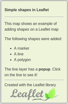
FIGURE 6.12: Map description

The above expression basically creates a <div> element with id="legend", then adds internal HTML content into that element. Adding the HTML code is done with the plain JavaScript .innerHTML method, which we met in Section 4.3.3. We could do the same with jQuery (Section 4.7.2), but it would not make the code much simpler in this case. Note that we are using the + operators in order to split the assigned HTML code string into multiple lines and make the code more manageable and easier to read. Finally, the control is added to the map with .addTo method, just like we did for map layers in previous examples in this chapter:

legend.addTo(map);

The complete code for adding the map description is as follows:

var legend = L.control({position: "bottomleft"});
legend.onAdd = function(map) {
    var div = L.DomUtil.create("div", "legend");
    div.innerHTML = 
        '<p><b>Simple shapes in Leaflet</b></p><hr>' +
        '<p>This map shows an example of adding shapes ' + 
        'on a Leaflet map</p>' +
        'The following shapes were added:<br>' +
        '<p><ul>' +
        '<li>A marker</li>' +
        '<li>A line</li>' +
        '<li>A polygon</li>' +
        '</ul></p>' +
        'The line layer has a <b>popup</b>. ' + 
        'Click on the line to see it!<hr>' +
        'Created with the Leaflet library<br>' +
        '<img src="images/leaflet.png">';
    return div;
};
legend.addTo(map);

We also need some CSS code to give our map description the final styling shown in Figure 6.12:

.legend {
    font-size: 16px;
    line-height: 24px;
    color: #333333;
    font-family: 'Open Sans', Helvetica, sans-serif;
    padding: 10px 14px;
    background-color: rgba(245,245,220,0.8) ;
    box-shadow: 0 0 15px rgba(0,0,0,0.2);
    border-radius: 5px;
    max-width: 250px;
    border: 1px solid grey;
}
.legend p {
    font-size: 16px;
    line-height: 24px;
}
.legend img {
    max-width: 200px;
    margin: auto;
    display: block;
}

Finally, we need to have the leaflet.png image file in the images sub-directory inside the directory where the HTML document is, for the last expression in our HTML code to work. The expression adds the Leaflet library logo in the bottom of the map description (Figure 6.12):

<img src="images/leaflet.png">

The resulting map example-06-07.html, with the map description information box in the bottom-left corner, is shown in Figure 6.13.

FIGURE 6.13: example-06-07.html (Click to view this example on its own)

6.9 Introducing map events

In Section 4.3.4, we learned how the browser fires events in response to user interactions, and that these events can be handled using JavaScript to make our web page interactive. We also mentioned the event object (Section 4.11), which can be used to trigger specific responses according to event properties. Recall the mouse position in example-04-07.html (Figure 4.8), where mouse position was printed on screen thanks to the pageX and pageY properties of the event object. In Section 4.11, we also mentioned that custom event types and custom event object properties are often defined in JavaScript libraries for specific needs.

The Leaflet library defines specific event types and event properties appropriate for web mapping. These specific events can be captured for the entire map object, or for specific features the map contains. In this context, a popup is an example of a built-in event listener, with a pre-defined behavior: opening on click, closing when the “X” button or any other layer is clicked. Similarly, we can define and customize other Leaflet map interactive behaviors.

One of the most useful types of map events are "click" events, and the most important property of a map click event is the spatial location where the user clicked. When the user clicks on the map—in addition to the usual "click" event properties—the event object contains the latitude and longitude of where the click was made. The latitude and longitude are given in the special .latlng property of the map event object. The .latlng event object property opens up the possibility of “capturing” the clicked coordinates and doing something useful with them.

For example, in Chapter 11 we will use the clicked location to query specific features—that are near the clicked location—from a database (Figure 11.8). In this section, we will see a simpler example, displaying the clicked coordinates inside a popup, which is opened on the clicked location itself (Figure 6.15). To display the currently clicked location using a popup, we need to do several things:

• Add an empty popup object to our map
• Write a function that, once called, sets popup location, fills the popup with content, and opens it on the map
• Add an event listener stating that each time the map is clicked, the latter function is executed

Starting with the first item, an empty popup object can be created with the L.popup function, as follows. This is in contrast to the .bindPopup method we used earlier to bind a popup to an existing layer (Section 6.7):

var popup = L.popup();

In the function that the event listener will refer to, hereby named onMapClick (see below), we will be using the event object parameter e. As mentioned above, when referring to map "click" events, the event object includes the .latlng property. The .latlng property is itself an object of type LatLng, which holds the longitude and latitude of the clicked location. This is basically a JavaScript object with two properties and two numeric values, such as the following one (plus some additional methods, which we don’t need to worry about at the moment):

{lat: 31.2596049045682, lng: 34.80215549468995}

A LatLng object can be created with L.latLng, and it can be used for specifying coordinates instead of a simple [lat, lon] array. For example, try running the following expression in the console in any of the above examples. This will add a marker at a location defined using a LatLng object:

L.marker(L.latLng(31.264, 34.802)).addTo(map);

Back to the event listener example. The LatLng object, representing the clicked location, will be used for two purposes:

• Determining where the popup should be opened
• Setting the popup contents

These are accomplished with two methods of the popup object, .setLatLng and .setContent. Finally, once popup placement and content are set, the popup will be opened using a third method named .openOn. The event listener function, hereby named onMapClick, thus takes the following form:

function onMapClick(e) {
    popup
        .setLatLng(e.latlng)
        .setContent(
            "You clicked the map at -<br>" + 
            "<b>lon:</b> " + e.latlng.lng + "<br>" + 
            "<b>lat:</b> " + e.latlng.lat
        )
        .openOn(map);
}

To better understand what this function does, try running the following code in the console in one of the Leaflet examples from this chapter:

var myLocation = L.latLng(31.264, 34.802);
L.popup()
    .setLatLng(myLocation)
    .setContent(
        "You clicked the map at -<br>" + 
        "<b>lon:</b> " + myLocation.lng + "<br>" + 
        "<b>lat:</b> " + myLocation.lat
    )
    .openOn(map);

This is basically the same code as the body of the onMapClick function, only that instead of e.latlng we used a specific LatLng instance, named myLocation. As a result of running this code section, you should see a popup with the content shown in Figure 6.14, opened at the location specified by L.latLng(31.264, 34.802).

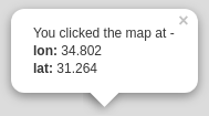
FIGURE 6.14: A popup displaying clicked location coordinates

Finally, we add an event listener specifying that the onMapClick function should be executed on map click. Note that in this case the element responding to the event is the entire map, so that any click inside the map triggers the onMapClick function:

map.on("click", onMapClick);

The complete code we need to add to a basic Leaflet map, so that clicked coordinates are displayed in a popup, is shown on the following page:

var popup = L.popup();
function onMapClick(e) {
    popup
        .setLatLng(e.latlng)
        .setContent(
            "You clicked the map at -<br>" + 
            "<b>lon:</b> " + e.latlng.lng + "<br>" + 
            "<b>lat:</b> " + e.latlng.lat
        )
        .openOn(map);
}
map.on("click", onMapClick);

The resulting map example-06-08.html is shown in Figure 6.15.

FIGURE 6.15: example-06-08.html (Click to view this example on its own)

• Open example-06-08.html (Figure 6.15) and click anywhere on the map.
• As shown in Figure 6.15, the popup displays the e.latlng coordinates “as is”, with many irrelevant digits.
• The first six digits refer to sub-meter (~0.1 m) precision, which is more than enough for most types of applications.
• Modify the onMapClick function so that the coordinates are rounded and only the first six digits of longitude and latitude are displayed inside the popup. (Hint: you can search on Google for a JavaScript function to round numbers according to specified number of digits.)

6.10 Exercise

• Create a Leaflet map with the location of places you want to visit, and the path you want to travel along between those places.
• The map should have the following components:
  • A tile layer
  • Markers of the visited locations
  • A line representing the travel path
  • Popups for each marker, containing location names
  • A description box, with your name and the list of locations in the right order
• Optional: Check out the Layer Groups and Layers Control tutorial, and try to add a layer control for showing or hiding the markers and the line layers, and for switching between two or more types of tile layers (Figure 6.16).

FIGURE 6.16: solution-06.html (Click to view this example on its own)

References

Crickard III, Paul. 2014. Leaflet. Js Essentials. Birmingham, UK: Packt Publishing Ltd.

Dincer, Alper, and Balkan Uraz. 2013. Google Maps Javascript Api Cookbook. Birmingham, UK: Packt Publishing Ltd.

Farkas, Gábor. 2016. Mastering Openlayers 3. Birmingham, UK: Packt Publishing Ltd.

Gratier, Thomas, Paul Spencer, and Erik Hazzard. 2015. OpenLayers 3: Beginner’s Guide. Packt Publishing Ltd.

Langley, Peter J, and Antonio Santiago Perez. 2016. OpenLayers 3.x Cookbook. 2nd ed. Birmingham, UK: Packt Publishing Ltd.

Murray, Scott. 2017. Interactive Data Visualization for the Web: An Introduction to Designing with D3. Sebastopol, CA, USA: O’Reilly Media, Inc.

Newton, Thomas, and Oscar Villarreal. 2014. Learning D3.js Mapping. Birmingham, UK: Packt Publishing Ltd.

Rubalcava, Rene. 2015. ArcGIS Web Development. Shelter Island, NY, USA.: Manning Publications Co.

---

46. A good introduction to web mapping can be found in the Web Maps 101 (http://maptimeboston.github.io/web-maps-101/#0) presentation by Maptime Boston (https://maptimeboston.github.io/resources).↩

47. Check out the What is a web mapping API? (https://www.e-education.psu.edu/geog585/node/763) article for additional information on pros and cons of different web-mapping libraries.↩

48. See Appendix A for complete list of files and directory structure; see online version (Section 0.7) for downloading the complete set of files for the Leaflet library.↩

49. You can always to refer to the documentation (https://leafletjs.com/reference-1.5.0.html) for the complete list of options for L.map, or any other Leaflet function.↩

50. See the Zoom levels tutorial (https://leafletjs.com/examples/zoom-levels/) for more information on tile layer zoom levels and their implementation in Leaflet.↩

51. Again, for the complete list of options see the Leaflet documentation (https://leafletjs.com/reference-1.5.0.html#tilelayer).↩

52. For more information, see the Leaflet on Mobile tutorial (https://leafletjs.com/examples/mobile/).↩

53. Remember that the coordinates arrays that Leaflet accepts follow the [lat, lon] format, not the [lon, lat] format!↩

54. The complete list of Leaflet layer types is given in the Leaflet documentation (https://leafletjs.com/reference-1.5.0.html).↩

55. See the Leaflet Quick Start Tutorial (https://leafletjs.com/examples/quick-start/) for another overview on adding simple layers with popups in Leaflet.↩

56. In subsequent chapters, we are going to use L.control to display other types of controls, such as a map legend (Section 8.6), a dynamically updated information box (Section 8.8.2), and a dropdown menu (Section 10.3).↩