Chapter 9 Geometric operations with rasters
Last updated: 2021-03-31 00:26:19
Aims
Our aims in this chapter are:
- Make changes in the geometric component of rasters:
- Mosaicking
- Resampling
- Reprojecting
- Apply focal filters on a raster
We will use the following R packages:
starsunits
9.1 Mosaicking rasters
In the next few examples, we will prepare a Digital Elevation Model (DEM) raster of Haifa, by mosaicking, subsetting and reprojecting (Section 9.3).
We start with two \(5°\times5°\) tiles of elevation data from the Shuttle Radar Topography Mission (SRTM) dataset. The tiles are included as two .tif files in the sample files (Appendix A):
library(stars)
dem1 = read_stars("srtm_43_06.tif")
dem2 = read_stars("srtm_44_06.tif")
As shown in Figure 9.1, the tiles cover the area of northern Israel, including Haifa:
plot(dem1, breaks = "equal", col = terrain.colors(10), axes = TRUE)
plot(dem2, breaks = "equal", col = terrain.colors(10), axes = TRUE)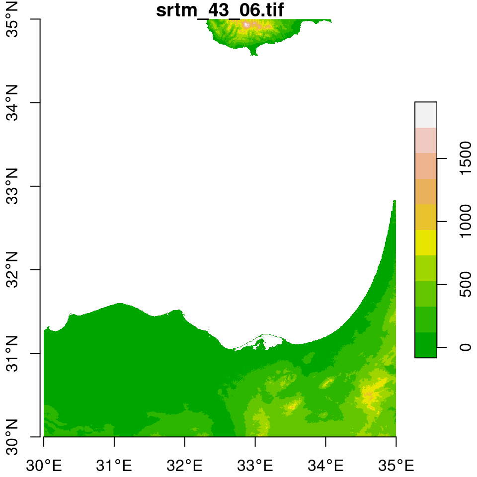
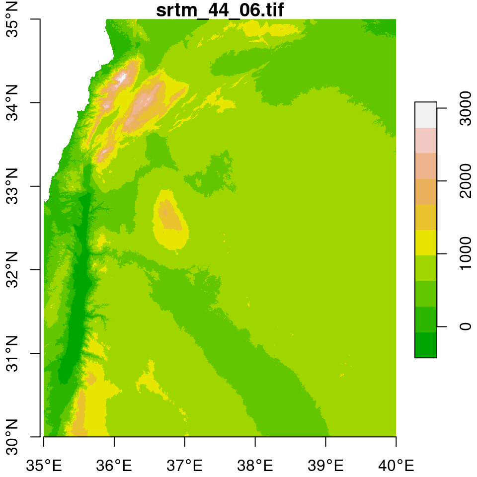
Figure 9.1: Two elevation tiles from the SRTM dataset
Using the st_bbox and dim functions (Section 5.3.8.3), we can see that the two rasters indeed comprise two tiles of the same “large” dataset. First, we can see that the dimensions (number of rows and columns) of the two rasters are identical:
dim(dem1)
##    x    y
## 6000 6000
dim(dem2)
##    x    y
## 6000 6000
Second, we can see that their extents of the rasters are aligned. The y-axis (i.e., latitude) extent of the rasters is the same (30-35). The x-axis (i.e., longitude) extents of the rasters are side-by-side (30-35 and 35-40):
st_bbox(dem1)
## xmin ymin xmax ymax
##   30   30   35   35
st_bbox(dem2)
## xmin ymin xmax ymax
##   35   30   40   35
Rasters can be mosaicked using the st_mosaic function. The st_mosaic function accepts two or more stars objects—such as dem1 and dem2—and returns a combined raster:
dem = st_mosaic(dem1, dem2)
names(dem) = "elevation"
Note that the st_moisaic function can be used to combine rasters even if they are not aligned, such as in this example. In case the rasters are not aligned, resampling (Section 9.2) take place.
The mosaicked DEM is shown in Figure 9.2:
plot(dem, axes = TRUE, breaks = "equal", col = terrain.colors(10))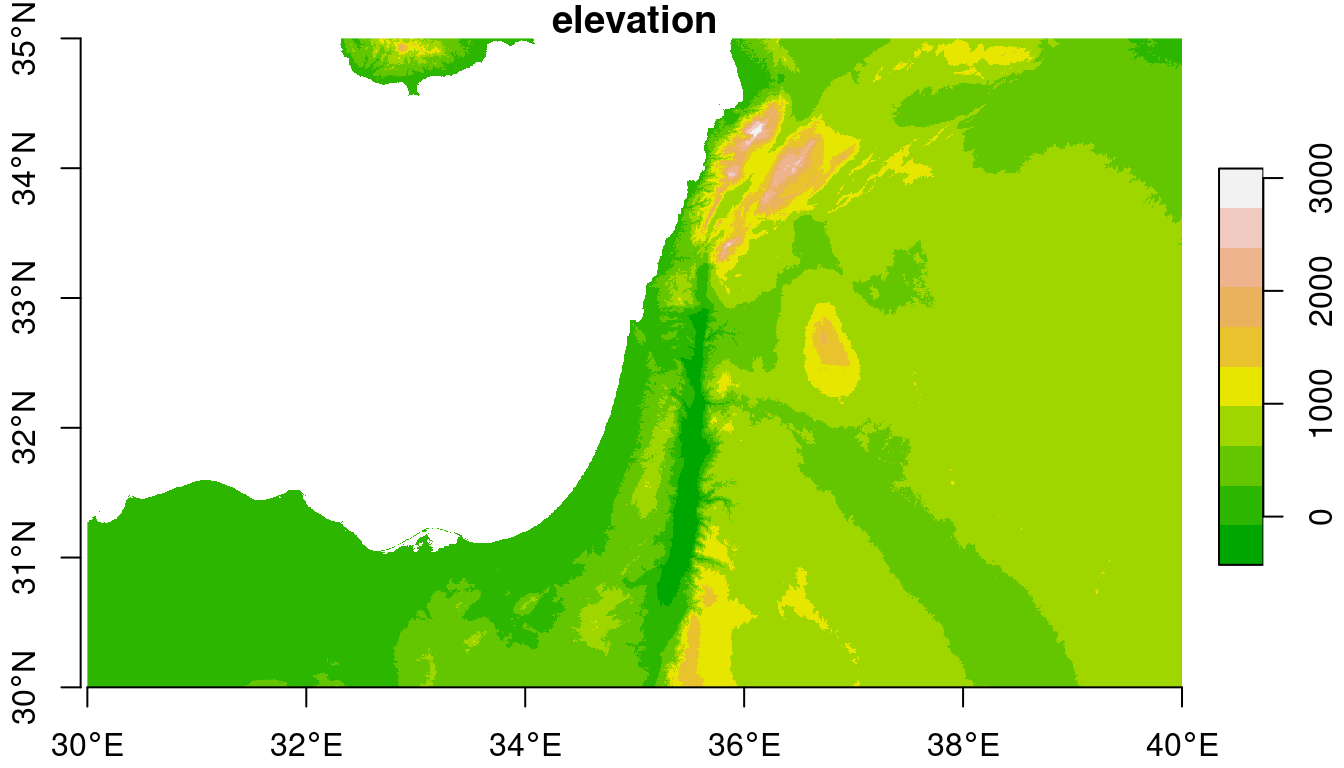
Figure 9.2: Mosaicked raster
The extent of the resulting raster covers the extents of both inputs:
st_bbox(dem)
## xmin ymin xmax ymax
##   30   30   40   35
For the next examples, we “crop” the dem raster according to an extent of \(0.25°\times0.25°\) around Haifa (Figure 9.3).
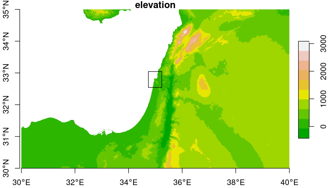
Figure 9.3: An \(0.25°\times0.25°\) rectangular extent
The [ operator can be used to crop the raster (Section 6.2):
dem = dem[, 5687:6287, 2348:2948]The result is shown in Figure 9.4:
plot(dem, axes = TRUE, breaks = "equal", col = terrain.colors(10))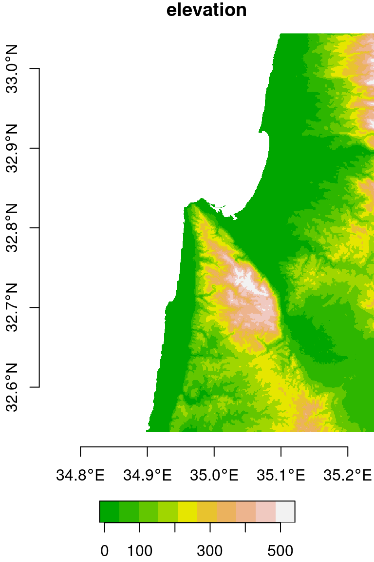
Figure 9.4: Cropped raster
Note that in this example, we needed to know in advance the row and column indices of the extent we are interested in cropping. Later on (Section 10.1), we are going to learn how to crop a raster based on an existing vector layer, such as the bounding box of a buffer of \(0.125°\) around a point layer representing the city of Haifa, which is a much more practical approach.
9.2 Raster resampling
9.2.1 The st_warp function
Raster resampling is the process of transferring raster values from the original grid to a different grid (Figure 9.5). Resampling is onften required for:
- Aligning several input rasters that come from different sources to the same grid, so that they can be subject to spatial operators such as raster algebra (Sections 6.4 and 6.6.1)
- Reducing the resolution of very detailed rasters, so that they are more convenient to work with in terms of processing time and memory use
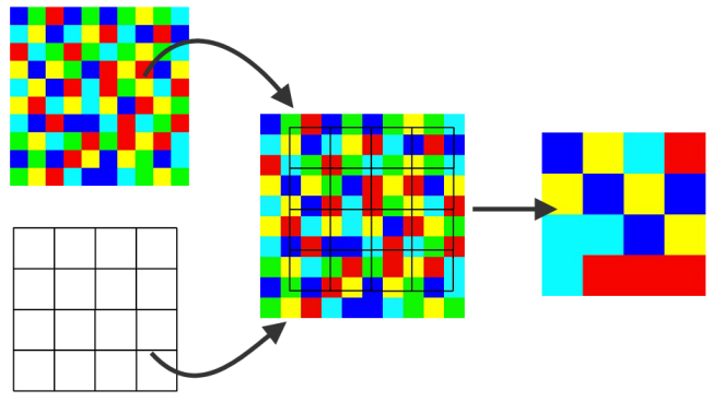
Figure 9.5: Raster resampling (https://www.safe.com/transformers/raster-resampler/)
To demonstrate resampling, we will create a custom stars grid, using the same extent as the dem raster (st_bbox(dem)), but a coarser resolution. The new resolution is \(0.002°\), which is ~2.4 times the original resolution of \(0.00083°\). The grid is created using st_as_stars:
grid = st_as_stars(st_bbox(dem), dx = 0.002, dy = 0.002)
grid
## stars object with 2 dimensions and 1 attribute
## attribute(s):
##     values
##  Min.   :0
##  1st Qu.:0
##  Median :0
##  Mean   :0
##  3rd Qu.:0
##  Max.   :0
## dimension(s):
##   from  to  offset  delta refsys point values x/y
## x    1 251 34.7383  0.002 WGS 84    NA   NULL [x]
## y    1 251 33.0442 -0.002 WGS 84    NA   NULL [y]
Recall that we already used the st_as_stars function to convert a matrix to a stars raster (Section 6.3.3). What we do here is another mode of operation of the st_as_stars function, creating an empty raster given a bbox and the x- and y-axis resolutions dx and dy.
We can resample a raster using the st_warp function. The first two parameters of st_warp are:
- The raster to be resampled, where the values come from
- The raster defining the new grid
Here is the expression to resample the values of the dem raster into the new raster grid:
dem1 = st_warp(dem, grid)Which one of the rasters in Figure 9.5 represents the role of
demandgrid, in our case?
Try resampling
demto a different grid with an even coarser resulution, such as0.02, and plot the result
The original DEM is shown along with the resampled one in Figure 9.6.
plot(dem, breaks = "equal", col = terrain.colors(10), main = "input (delta=0.0008)")
plot(dem1, breaks = "equal", col = terrain.colors(10), main = "output (delta=0.002)")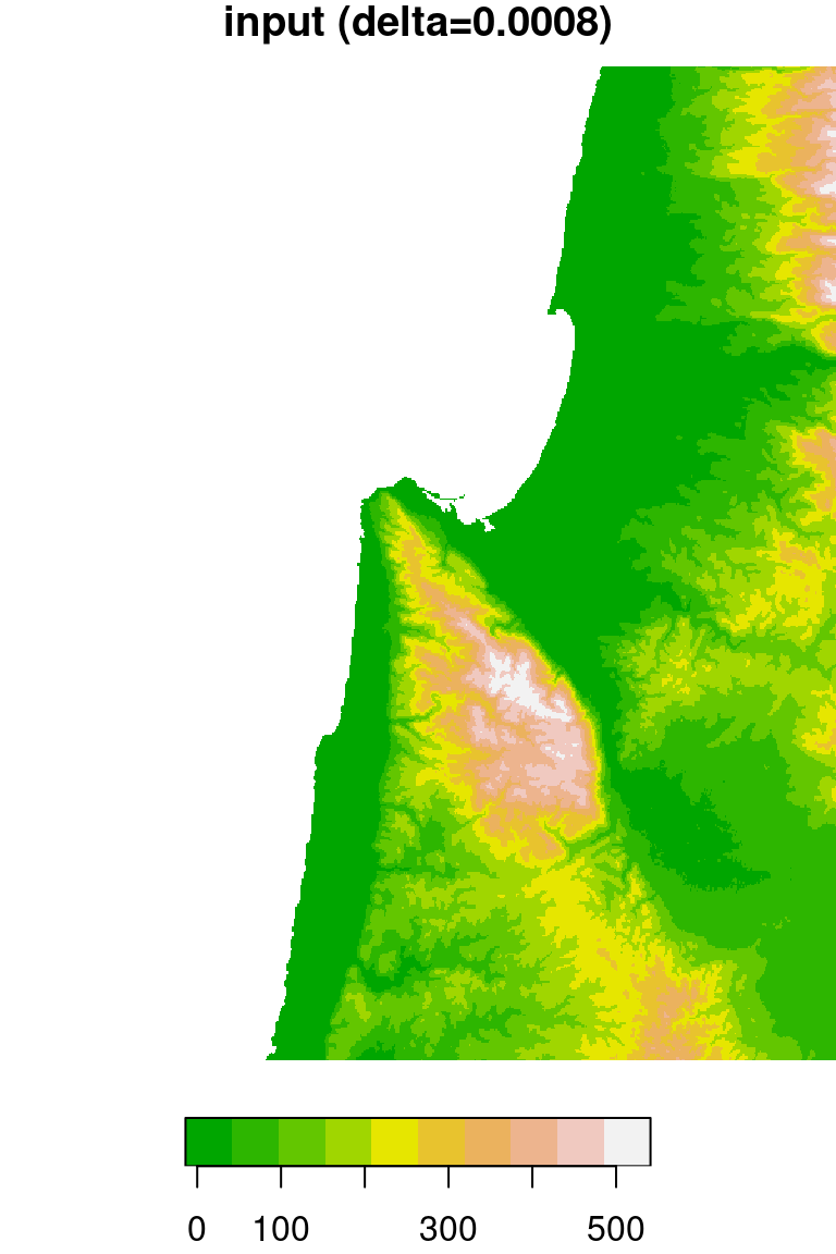

Figure 9.6: DEM resampled by a factor of 2.4, from 0.0008 (left) to 0.002 (right) resolution
When resampling, the computer needs to decide which pixel value(s) to transfer to each of the “new” pixels, defined by the new grid. There are several possible options, known as resampling algorithms or methods. In the next three sections, we are going to demonstrate three common options:
9.2.2 Nearest neighbor resampling
The st_warp expression from Section 9.2.1 actually used the nearest neighbor resampling method (method="near"), which is the default:
dem1 = st_warp(dem, grid, method = "near")To understand what actually happens in nearest neighbor resampling, let’s take a look at a small part of the raster “before” and “after” images (Figure 9.7). If you look closely, you can see that the values of the original raster are passed to the resampled raster. What happens when there is more than one pixel of the original raster coinciding with a single pixel in the new grid? How can we decide which value is going to be passed? In nearest neighbor resampling, the new raster pixels get the value from the nearest pixel of the original raster. Note that some of the values may be “lost” this way, since they were not passed on to the new raster32.
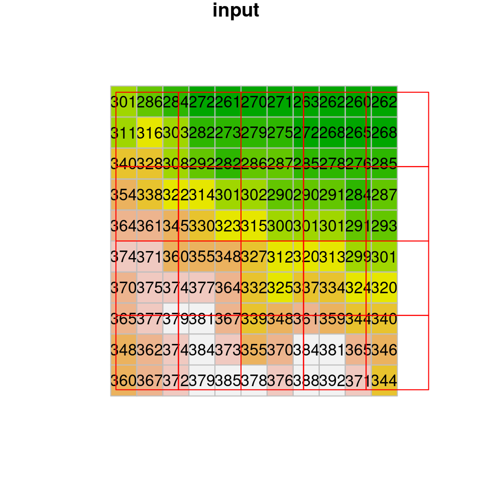
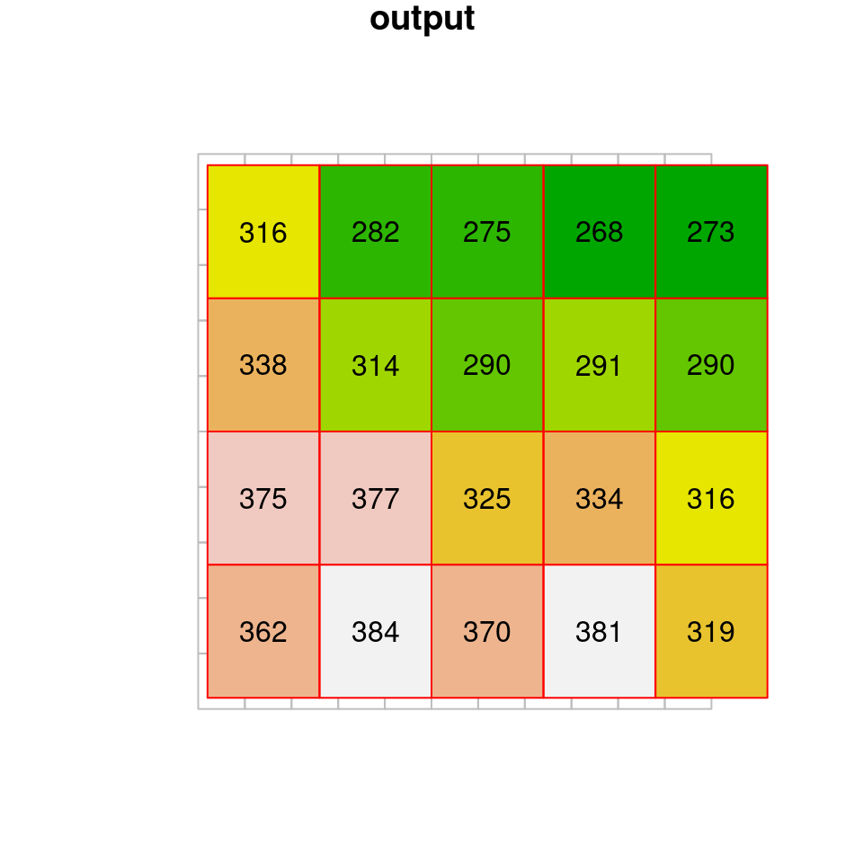
Figure 9.7: Nearest neighbor resampling
9.2.3 Bilinear resampling
Bilinear resampling is another resampling method. In bilinear resampling, each new raster cell gets a weighted average of four nearest cells from the input, rather than just one. Bilinear resampling is specified with method="bilinear" in st_warp. Note that use_gdal=TRUE needs to be specified when using any method other than method="near", otherwise the method argument is ignored:
dem1 = st_warp(dem, grid, method = "bilinear", use_gdal = TRUE)With bilinear resampling, the output raster is “smoothed,” containing new values which are averages of (some of) the values in the original raster (Figure 9.8).

Figure 9.8: Bilinear resampling
9.2.4 Average resampling
Another useful method is the average resampling method, where each new cell gets the weighted average of all overlapping input cells:
dem1 = st_warp(dem, grid, method = "average", use_gdal = TRUE)The result of average resampling is shown in Figure 9.9:

Figure 9.9: Average resampling
In addition to "near", "bilinear", and "average", the st_warp function supports other resampling methods, including: "cubic", "cubicspline", "lanczos", "mode", "max", "min", "med", "q1" and "q3".
Bilinear resampling may be preferred when the result is primarily used for visualization, because the result appears smoother. Nearest neighbor resampling, however, is preferable when we are using the result for further analysis, because the original values are preserved. When the input raster is categorical, such as a raster with land cover classes 1, 2, 3, etc., nearest neighbor resampling is the only valid resampling option, because averaging category IDs makes no sense.
In what situations do you think the
"average"resampling method is mostly appropriate, while"near"and"bilinear"are not?
9.3 Raster reprojection
Raster reprojection is more complex than vector layer reprojection (Section 7.9.2). In addition to transforming (pixel) coordinates, like in vector layer reprojection, raster reprojection requires a resampling step in order to “arrange” the transformed values back into a regular grid (Figure 9.14).
In terms of code, the st_warp function, which we used for resampling (Section 9.2), is used for raster reprojection too. The only difference is that, in raster reprojection, the “destination” grid is specified in a different CRS.
For example, the following expression reprojects the DEM of Haifa from WGS84 (4326) to UTM (32636), using the nearest neighbor resampling method. Note that, in this example, we are not passing a stars object with the destination grid. Instead, we are letting the function to automatically generate the new grid, only specifying the destination CRS (crs=32636) and resolution (cellsize=90):
dem = st_warp(dem, crs = 32636, cellsize = 90)The original raster (in WGS84) and the reprojected one (in UTM) are shown in Figure 9.10.
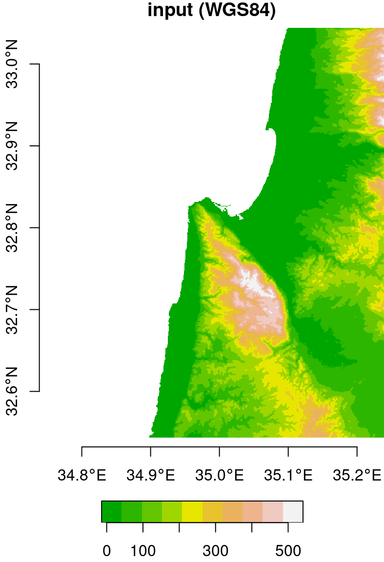
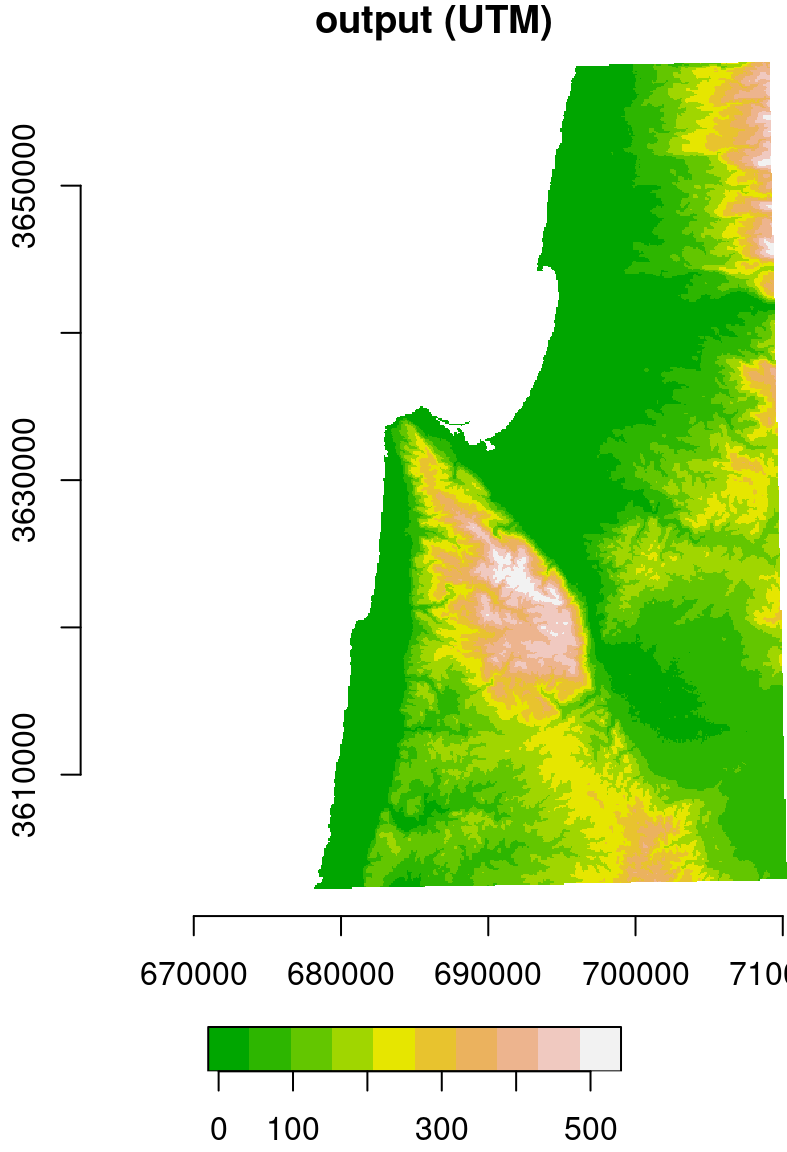
Figure 9.10: Original (left, in WGS84) and reprojected (right, in UTM) dem raster
Note that the coordinate units in the reprojected raster (Figure 9.10) are no longer degrees, but meters. Also, the area contaning non-missing values is slightly rotated compared to the input, because the WGS84 and UTM systems are not parallel, at least in this particular location.
A zoomed-in view (Figure 9.11) of the original raster and the new grid demonstrates that the two are not parallel. Again, note that this time the new grid is in a different CRS, which is why the two grids are not parallel to each other (Figure 9.7–9.9).
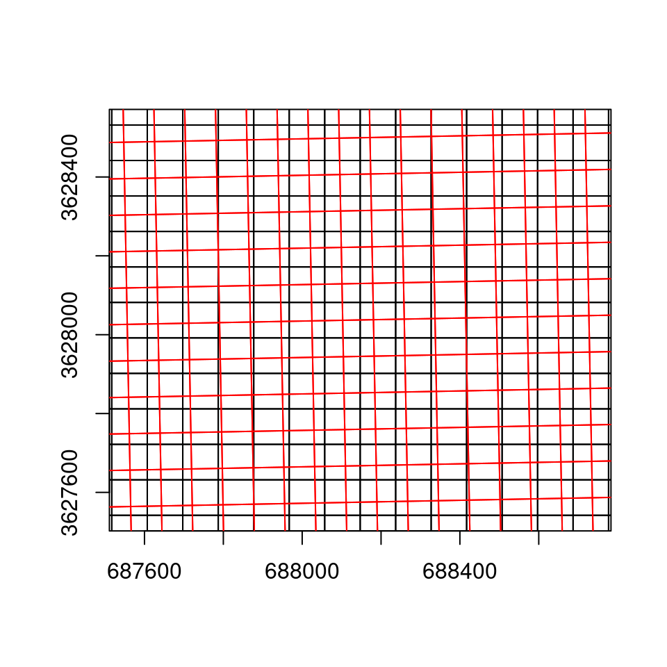
Figure 9.11: The reprojected raster grid (UTM, black) and the original raster grid (WGS84, in red), displayed in UTM
As another example, let’s reproject the MOD13A3_2000_2019.tif, from its sinusoidal projection to a projection more suitable for the specific region, such as ITM (Table 7.4). First, let’s import the raster from the GeoTIFF file:
r = read_stars("MOD13A3_2000_2019.tif")
names(r) = "NDVI"
Then, we can reproject the raster using st_warp. This time we specify just the destination CRS (crs=2039), letting the function automatically determine the resolution:
r_itm = st_warp(r, crs = 2039)The original and reprojected rasters are shown in Figure 9.12:
plot(r[,,,1,drop=TRUE], key.pos = 4, axes = TRUE, col = hcl.colors(11, "Spectral"), main = "input (Sinusoidal)")
plot(r_itm[,,,1,drop=TRUE], key.pos = 4, axes = TRUE, col = hcl.colors(11, "Spectral"), main = "output (ITM)")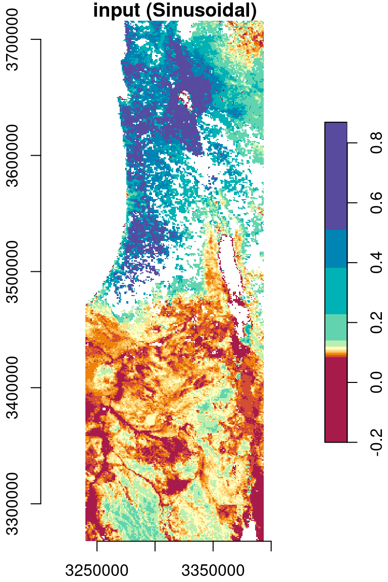
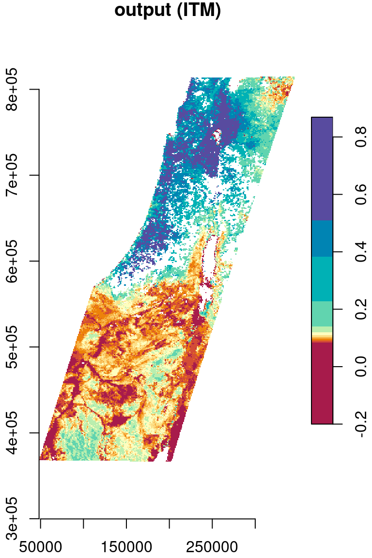
Figure 9.12: Reprojection of the MODIS NDVI raster from Sinusoidal (left) to ITM (right)
To see the process of reprojection more clearly, let’s examine a small subset of the NDVI raster:
u = r[, 100:105, 200:207, 2, drop = TRUE]
u_itm = st_warp(u, crs = 2039)
The original and reprojected raster subsets are shown in Figure 9.13.
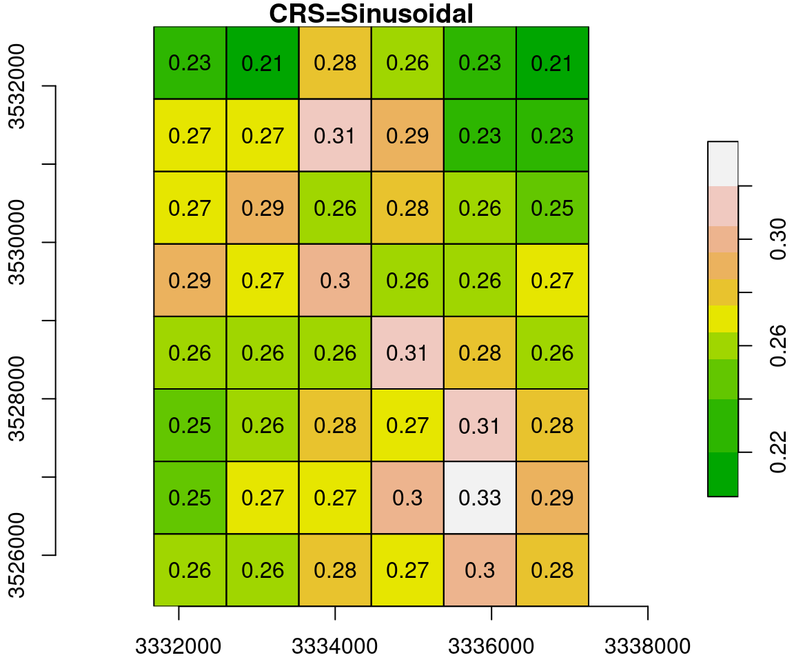
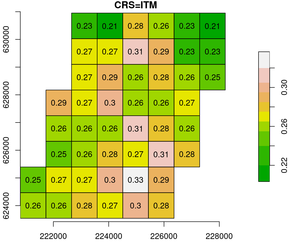
Figure 9.13: Reprojection of a small subset of the MODIS NDVI raster (left) to ITM (right)
What happens in the reprojection can be thought of as a two-step process (Figure 9.14). In the first step, the pixel outlines are reprojected as if they were polygons (Section 7.9.2), which results in an irregular grid. The grid is then resampled (Section 9.2) to form a regular grid, so that it can be represented by a raster once again.
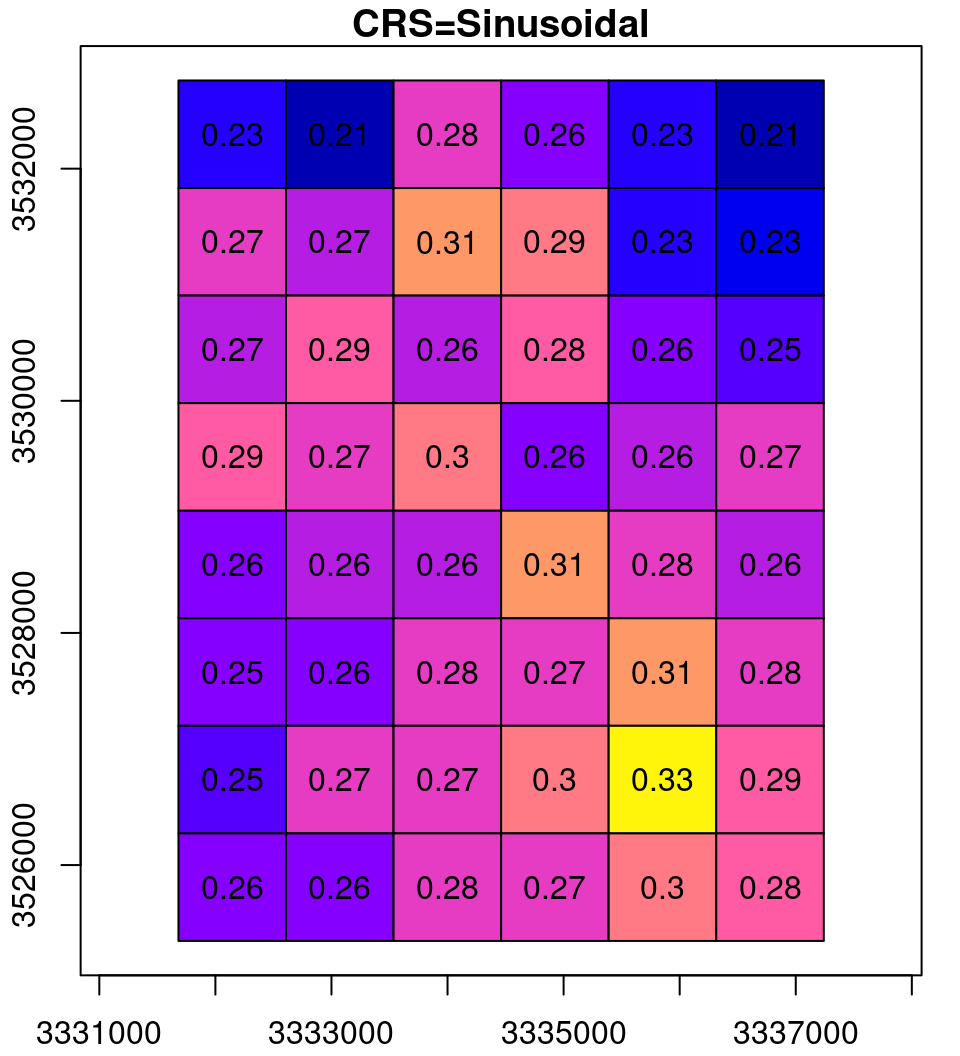
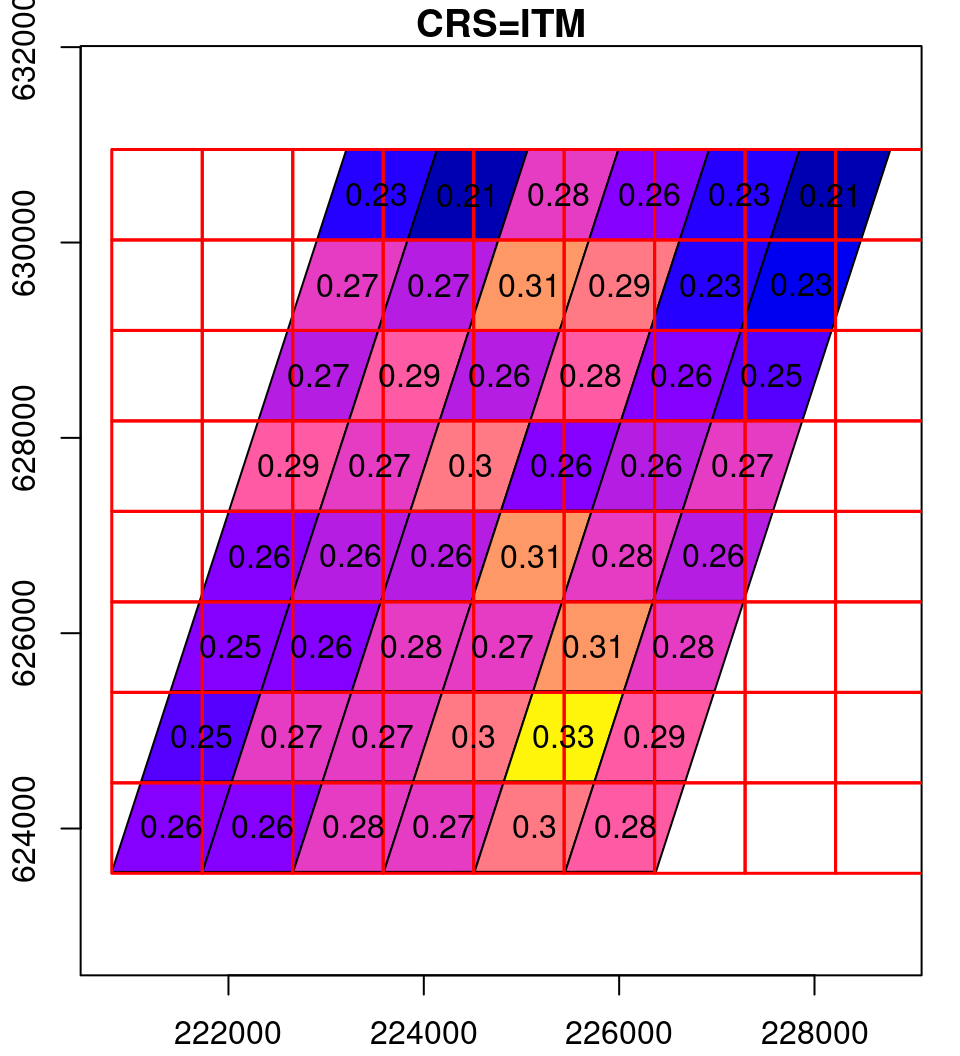
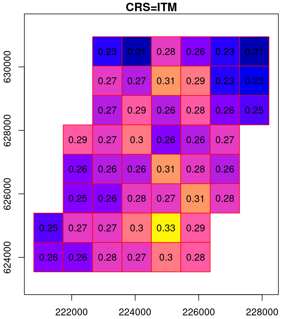
Figure 9.14: Reprojection process: the original raster (left), the reprojected raster cells as polygons (middle) and the resampled reprojected raster (right)
9.4 Focal filters
9.4.1 Introduction
So far, we only dealt with arithmetic operations that address the values of each per pixel in isolation from neighboring pixels, such as in raster algebra (Sections 6.4 and 6.6.1). Another class of raster operations is where the calculation of each pixels depends on values of neighboring cells.
The most prominent example of a raster calculation based on neighboring cells is moving window calculations, also known as applying a focal filter. With a moving window calculation, raster values are transformed based on the values from a neighborhood surrounding each pixel. The functions applied on the neighborhood are varied, from simple functions such as mean for a low-pass filter (Section 9.4.2) to more complex functions, such as those used to calculate topographic slope and aspect (Section 9.4.4–9.4.5).
For example, a \(3\times3\) mean filter applied on a raster results in a new raster, where the values are averages of \(3\times3\) neighborhoods centered on that pixel. In Figure 9.15, the highlghted value in the output on the right (18.7) is the average of the highlighted \(3\times3\) neighborhood of the input on the left:
mean(c(27, 8, 22, 16, 21, 16, 6, 44, 8))
## [1] 18.66667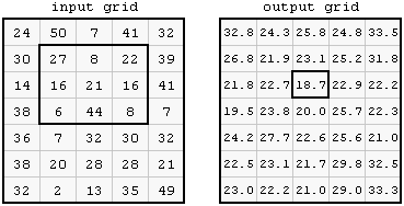
Figure 9.15: Focal filter (http://courses.washington.edu/gis250/lessons/raster_analysis1/index.html)
9.4.2 Low pass filter
9.4.2.1 What is a low pass filter?
The purpose of the mean, or low-pass, filter (Figure 9.15) is to produce a smoothed image, where extreme values (possibly noise) are cacelled out. For example, the result of applying a \(3\times3\) mean filter on a uniform image with one extreme value is shown in Figure 9.16.
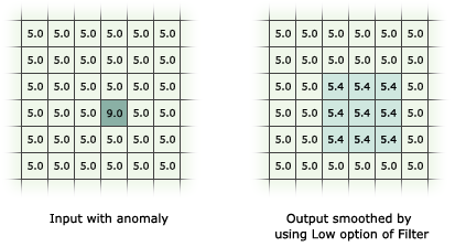
Figure 9.16: Low pass filter excample (http://desktop.arcgis.com/en/arcmap/10.3/tools/spatial-analyst-toolbox/how-filter-works.htm)
How was the value of
5.4obtained, in the result shown in Figure 9.16?
The stars package does not, at the moment, contain a function for focal filtering33. As an exercise, we are going to create our own function for focal filtering. For simplicity, we will restrict ourselves to the case where the focal “window” is \(3\times3\) pixels—which is the most common case.
Our working plan is as follows:
- Write a function named
get_neighborsthat accepts a position of the focal cell (row & column) in amatrix, and returns the 9 values of its \(3\times3\) pixel neighborhood - Write another function named
focal2that accepts a two-dimensionalstarsobject and a functionfun, iterates over the cells and appliesfunon all \(3\times3\) pixel neighborhoods extracted usingget_heighbors
9.4.2.2 The get_neighbors function
We start with a function that accepts a position (row & column) in a matrix and returns a numeric vector with the \(3\times3\) neighborhood, hereby named get_neighbors. The function accepts a matrix m and a position pos. The pos argument is a vector of length two, of the form c(row,column). The function extracts the 9 values in the respective \(3\times3\) neighborhood and returns them as a vector of length 9:
get_neighbors = function(m, pos) {
  i = (pos[1]-1):(pos[1]+1)
  j = (pos[2]-1):(pos[2]+1)
  as.vector(t(m[i, j]))
}
For example, suppose we have a \(5\times5\) matrix m:
m = matrix(1:25, ncol = 5, nrow = 5)
m
##      [,1] [,2] [,3] [,4] [,5]
## [1,]    1    6   11   16   21
## [2,]    2    7   12   17   22
## [3,]    3    8   13   18   23
## [4,]    4    9   14   19   24
## [5,]    5   10   15   20   25
Using get_neighbors, we can get the values of just about any \(3\times3\) neighborhood except for the outermost rows and columns (see below). For example, the following expression returns the values of the neighborhood centered on row 3, column 4:
get_neighbors(m, c(3, 4))
## [1] 12 17 22 13 18 23 14 19 24
How does the get_neighbors function work? The function first calculates the required range of rows and columns:
pos = c(3, 4)i = (pos[1]-1):(pos[1]+1) # Rows
i
## [1] 2 3 4j = (pos[2]-1):(pos[2]+1) # Columns
j
## [1] 3 4 5Then, the function extracts the corresponding matrix subset:
m[i, j]
##      [,1] [,2] [,3]
## [1,]   12   17   22
## [2,]   13   18   23
## [3,]   14   19   24
transposes it:
t(m[i, j])
##      [,1] [,2] [,3]
## [1,]   12   13   14
## [2,]   17   18   19
## [3,]   22   23   24
and converts to a vector:
as.vector(t(m[i, j]))
## [1] 12 17 22 13 18 23 14 19 24
Transposing is necessary so that the matrix values are returned by row, rather than the default by column (Section 5.1.4.1).
Note that out function is not designed to operate on the matrix edges, where the \(3\times3\) neighborhood is incomplete. For example, the following expression produces an error:
get_neighbors(m, c(1, 5))
## Error in m[i, j]: subscript out of bounds
9.4.2.3 The focal2 function
Now, let’s see how we can use the get_neighbors function to apply a focal filter on a raster. We will use the dem.tif small DEM for demonstration:
x = read_stars("dem.tif")First, we create a copy of the raster, named template. The template raster will be used as a “template” when converting the filtered matrix back to a stars object:
template = xNext, we extract the raster values as a matrix:
input = t(template[[1]])Note that the function relies on the fact that the stars object has just two dimensions (x and y), in which case input is going to be a matrix. The matrix is transposed, using t, to maintain the right orientation of the values matrix (Figure 6.11). This is important when using functions that distinguish between the north-south and east-west directions, topographic aspect (Section 9.4.5).
Next, we create another matrix to hold the output values. The values are initially set to NA:
output = matrix(NA, nrow = nrow(input), ncol = ncol(input))Now comes the actual computation. We are using two for loops to go over all raster cells, excluding the first and last rows and columns. For each cell, we:
- extract the \(3\times3\) neighborhood
[i,j], - apply a function—such as
mean, in this case—on the vector of extracted values, and - place the result into the corresponding cell
[i,j]in the output.
The complete code of the for loops is as follows:
for(i in 2:(nrow(input) - 1)) {
  for(j in 2:(ncol(input) - 1)) {
    v = get_neighbors(input, c(i, j))
    output[i, j] = mean(v, na.rm = TRUE)
  }
}
Note that the function starts at row i=2 and ends at row i=nrow(input)-1. Similarly, it starts at column j=2 and ends at j=ncol(input)-1.
In the end, when both for loops have been completed, the output matrix contains the new, filtered, raster values. What is left to be done is to put the matrix of new values into the template, to get back a stars object. We are using t once again, to transform the matrix back into the “stars” arrangement (Figure 6.11):
template[[1]] = t(output)The original image (x) and the filtered image (template) are shown in Figure 9.17. The figure highlights one \(3\times3\) neighborhood in the input, and the corresponding average of that neighborhood in the output34.
col = terrain.colors(5)
plot(x, text_values = TRUE, col = col, key.pos = 4, reset = FALSE, main = "input")
plot(st_geometry(st_as_sf(x, na.rm = FALSE)), border = "grey", add = TRUE)
plot(st_geometry(st_as_sf(x[,4:6,6:8])), lwd = 2, add = TRUE)
plot(round(template, 1), text_values = TRUE, col = col, key.pos = 4, reset = FALSE, main = "output")
plot(st_geometry(st_as_sf(template, na.rm = FALSE)), border = "grey", add = TRUE)
plot(st_geometry(st_as_sf(template[,5,7])), lwd = 2, add = TRUE)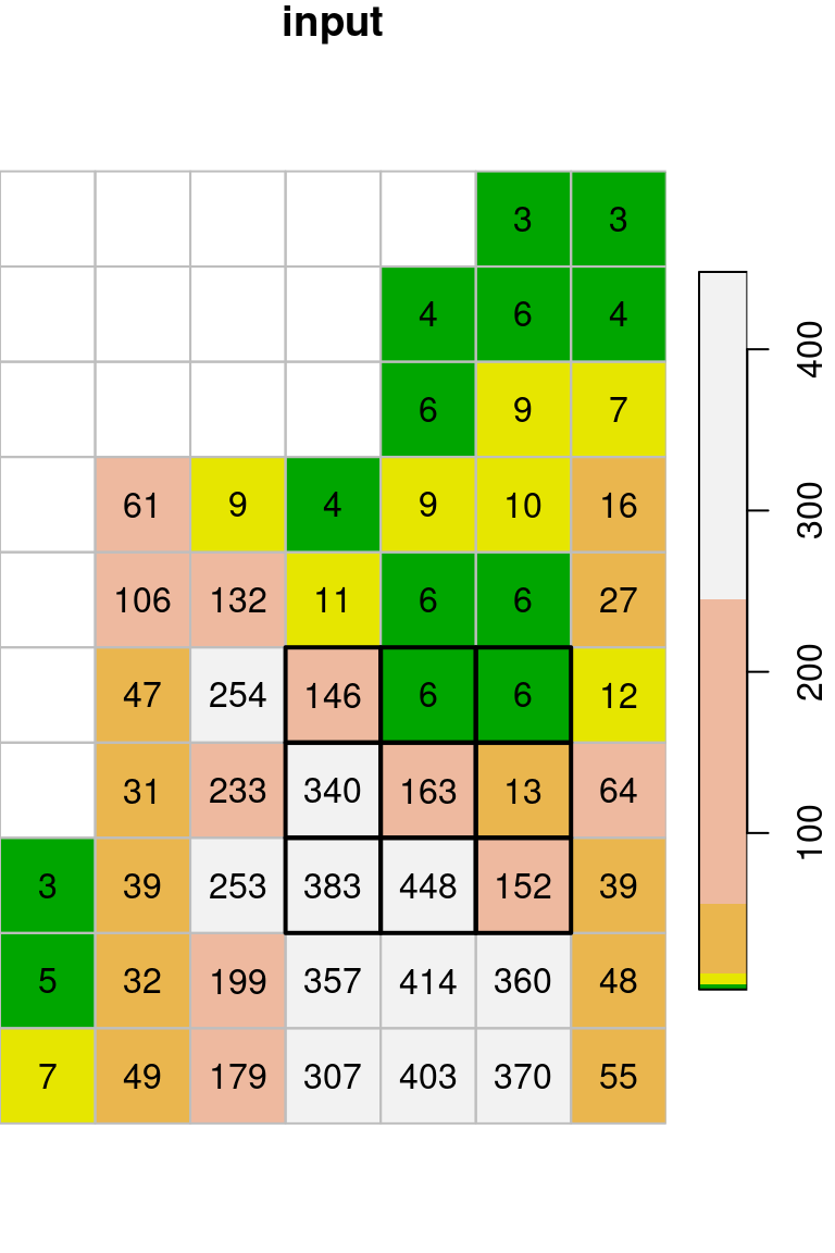
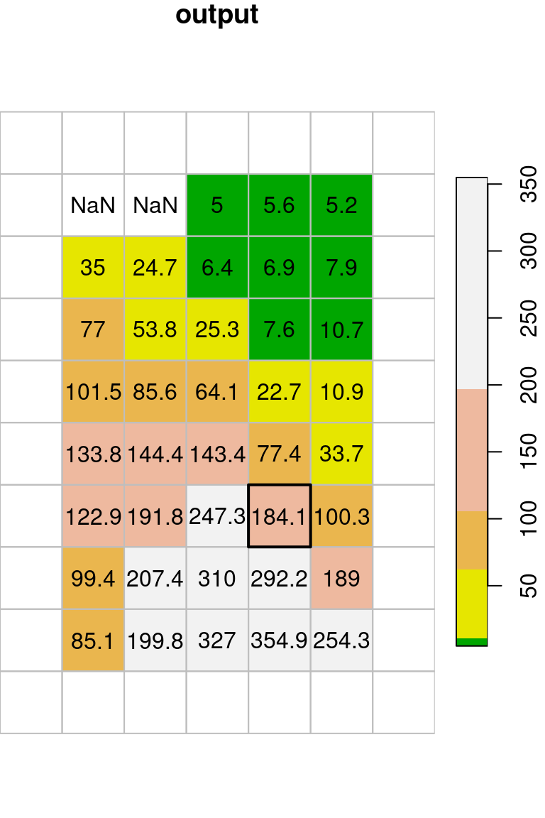
Figure 9.17: Focal filter with the mean function (left: input, right: result)
Why do the outermost rows and columns in Figure 9.17 appear empty? Which value do these pixels contain, and where did it come from?
Let’s manually check the calculation of the \(3\times3\) neighborhood highlighted in Figure 9.17:
t(x[[1]][4:6,6:8])
##      [,1] [,2] [,3]
## [1,]  146    6    6
## [2,]  340  163   13
## [3,] 383 448 152mean(t(x[[1]][4:6,6:8]))
## [1] 184.1111Why do you think we got
NaNvalues in some of the cells? Can you simulate the situation to see how anNaNvalues is produced? What can we do to getNA, instead, in those pixes that getNaN?
Wrapping up out code in a function, called focal2, can be done as follows. The input raster and the function are replaced with parameters named r and fun, respectively:
focal2 = function(r, fun) {
  template = r
  input = t(template[[1]])
  output = matrix(NA, nrow = nrow(input), ncol = ncol(input))
  for(i in 2:(nrow(input) - 1)) {
    for(j in 2:(ncol(input) - 1)) {
      v = get_neighbors(input, c(i, j))
      output[i, j] = fun(v)
    }
  }
  template[[1]] = t(output)
  return(template)
}
How can we pass additional parameters to the function we use, such as na.rm=TRUE for mean? The special dots ... argument is used for that. Now, any additional argument(s) passed to focal2 (such as na.rm=TRUE) will be passed on as additional argument(s) to fun:
focal2 = function(r, fun, ...) {
  template = r
  input = t(template[[1]])
  output = matrix(NA, nrow = nrow(input), ncol = ncol(input))
  for(i in 2:(nrow(input) - 1)) {
    for(j in 2:(ncol(input) - 1)) {
      v = get_neighbors(input, c(i, j))
      output[i, j] = fun(v, ...)
    }
  }
  template[[1]] = t(output)
  return(template)
}
Now that we have a custom focal filter function focal2, let’s try to apply a different filter, such as a maximum filter:
x_max = focal2(x, max, na.rm = TRUE)
## Warning in fun(v, ...): no non-missing arguments to max; returning -Inf

## Warning in fun(v, ...): no non-missing arguments to max; returning -Inf
The reason for the warnings produced by the above expression is that max applied on an empty vector gives -Inf.
t(x_max[[1]])
##       [,1] [,2] [,3] [,4] [,5] [,6] [,7]
##  [1,]   NA   NA   NA   NA   NA   NA   NA
##  [2,]   NA -Inf -Inf    6    9    9   NA
##  [3,]   NA   61   61    9   10   16   NA
##  [4,]   NA  132  132  132   11   27   NA
##  [5,]   NA  254  254  254  146   27   NA
##  [6,]   NA  254  340  340  340  163   NA
##  [7,]   NA  254  383  448  448  448   NA
##  [8,]   NA  253  383  448  448  448   NA
##  [9,]   NA  253  383  448  448  448   NA
## [10,]   NA   NA   NA   NA   NA   NA   NA
To get NA instead, we can use a slightly more complex function that first checks if particular neighborhood contains any non-NA values, any only then applies max:
f = function(x) if(all(is.na(x))) NA else max(x, na.rm = TRUE)
x_max = focal2(x, f)
Recall that we used the same principle when applying the min and max functions with st_apply (Section 6.6.1.4).
The resulting raster x_max is shown in Figure 9.18. Indeed, every pixel value in the output raster is the maximal value among the values in its \(3\times3\) neighborhood:
col = terrain.colors(10)
plot(x, text_values = TRUE, breaks = "equal", col = col, key.pos = 4, reset = FALSE, main = "input")
plot(st_geometry(st_as_sf(x, na.rm = FALSE)), border = "grey", add = TRUE)
plot(st_geometry(st_as_sf(x[,4:6,6:8])), lwd = 2, add = TRUE)
plot(x_max, breaks = "equal", text_values = TRUE, col = col, key.pos = 4, reset = FALSE, main = "output")
plot(st_geometry(st_as_sf(x_max, na.rm = FALSE)), border = "grey", add = TRUE)
plot(st_geometry(st_as_sf(x_max[,5,7])), lwd = 2, add = TRUE)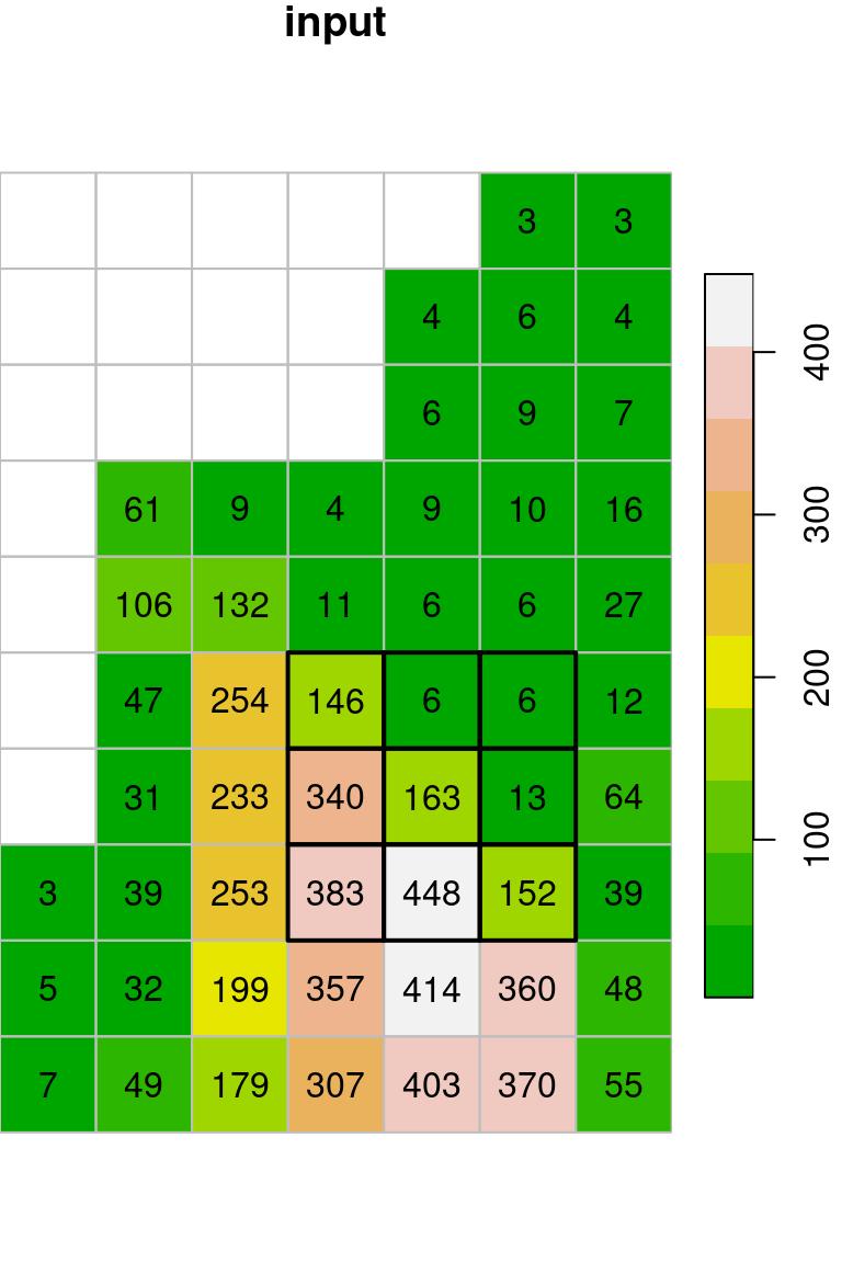
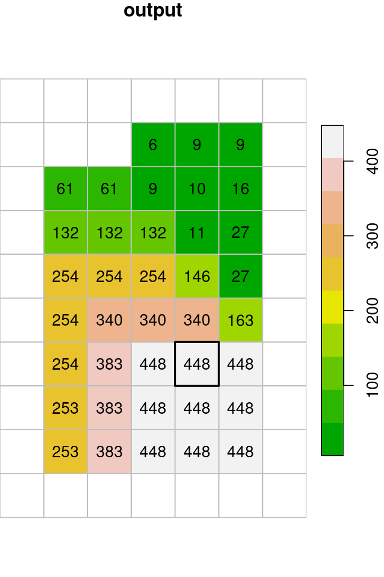
Figure 9.18: Focal filter with the max function (left: input, right: result)
Let’s try the focal2 function on another, bigger raster. For example, we can apply a low pass (i.e., mean) filter on the first layer of the MODIS NDVI raster, as follows:
r_itm1 = r_itm[,,,1,drop=TRUE]
r_itm1_mean = focal2(r_itm1, mean, na.rm = TRUE)
The original image and the filtered result are shown in Figure 9.19:
plot(r_itm1, col = hcl.colors(11, "Spectral"), main = "input")
plot(r_itm1_mean, col = hcl.colors(11, "Spectral"), main = "output")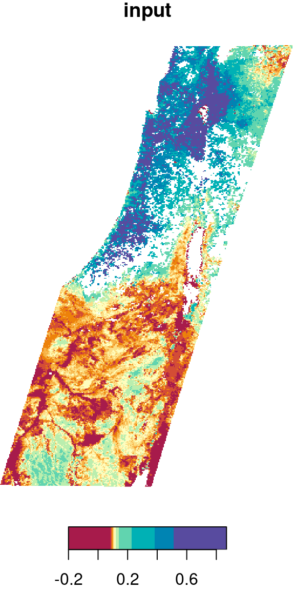
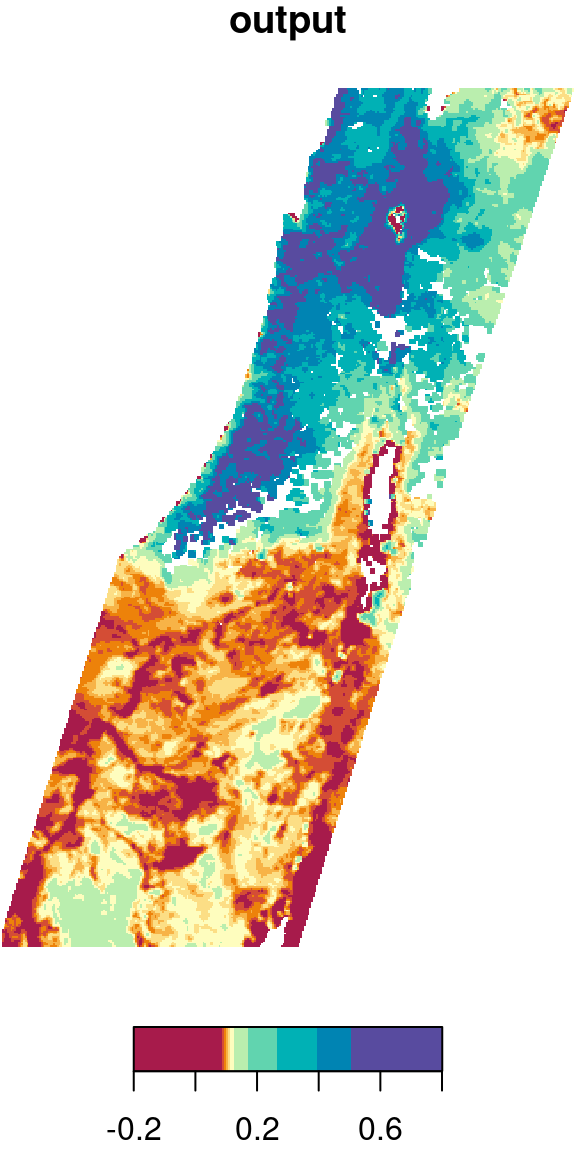
Figure 9.19: Low pass filter result
Why are there
NAareas in the raster, even though we usedna.rm=TRUE?
9.4.3 Maximum filter
For another example, let’s reconstruct the l_rec raster (Section 6.5):
l = read_stars("landsat_04_10_2000.tif")
red = l[,,,3, drop = TRUE]
nir = l[,,,4, drop = TRUE]
ndvi = (nir - red) / (nir + red)
names(ndvi) = "NDVI"
l_rec = ndvi
l_rec[l_rec < 0.2] = 0
l_rec[l_rec >= 0.2] = 1
Given a raster with 0 and 1 values, such as l_rec, we may want to convert all 0 cells neighboring to a 1 cell to become 1. That way, for instance, the areas of the planted forests we see in the center of the image will be come more continuous, which will make it easier to transform those areas into polygons (Section 10.3.2). This can be achieved with a focal filter and the max function:
l_rec_focal = focal2(l_rec, max)The original raster and the filtered result are shown in Figure 9.20:
plot(l_rec, col = c("grey90", "darkgreen"), main = "input")
plot(l_rec_focal, col = c("grey90", "darkgreen"), main = "output")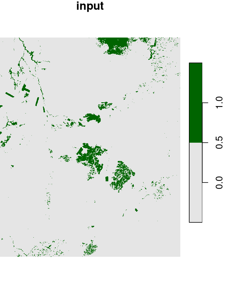
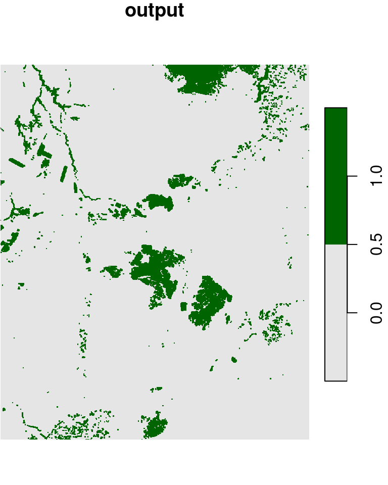
Figure 9.20: “Buffering” 1 values in a raster with 0s and 1s, using a focal filter with max
9.4.4 Topographic slope
So far we saw examples where the focal function is a simple built-in one, such as mean or max. In some cases, it is required to use a more complex function. For example, topographic indices such as slope and aspect employ complex functions where direction matters: each of the nine pixels in the \(3\times3\) neignborhood is treated differently.
For example, to calculate topographic slope based on elevation values in a \(3\times3\) neignborhood, the following function can be used. Note that the slope calulation also depends on raster resolution, which is passed as an additional parameter named res:
slope = function(x, res) {
  dzdx = ((x[3] + 2*x[6] + x[9]) - (x[1] + 2*x[4] + x[7])) / (8 * res)
  dzdy = ((x[7] + 2*x[8] + x[9]) - (x[1] + 2*x[2] + x[3])) / (8 * res)
  atan(sqrt(dzdx^2 + dzdy^2)) * (180 / pi)
}
We will not go into details on how the function works. You may refer to the How slope works article in the ArcGIS documentation for an explanation.
For example:
x = c(50, 45, 50, 30, 30, 30, 8, 10, 10)
res = 5
slope(x, res)  # 75.25762
## [1] 75.25766
The slope function can be passed to focal2 to apply the slope calculation on the entire dem raster:
dem_slope = focal2(dem, slope, res = st_dimensions(dem)$x$delta)
names(dem_slope) = "slope"
It is also convenient to set raster units with set_units (Section 8.3.2.2). The units of slope are decimal degrees (°):
library(units)
dem_slope[[1]] = set_units(dem_slope[[1]], "degree")
The resulting topographic slope raster is shown in the left panel in Figure 9.21.
9.4.5 Topographic aspect
Another function, as shown below, can be used to calculate topographic aspect:
aspect = function(x, res) {
  dzdx = ((x[3] + 2*x[6] + x[9]) - (x[1] + 2*x[4] + x[7])) / 8
  dzdy = ((x[7] + 2*x[8] + x[9]) - (x[1] + 2*x[2] + x[3])) / 8
  a = (180 / pi) * atan2(dzdy, -dzdx)
  if(is.na(a)) return(NA)
  if (a < 0) a = 90 - a else
    if (a > 90) a = 360 - a + 90 else
      a = 90 - a
  return(a)
}
For details on how the function works, see the How aspect works article in the ArcGIS documentation.
For example:
x = c(101, 92, 85, 101, 92, 85, 101, 91, 84)
aspect(x)  # 92.64
## [1] 92.64255
Again, the aspect function can be passed to focal2 to apply it on the entire raster:
dem_aspect = focal2(dem, aspect)
names(dem_aspect) = "aspect"
dem_aspect[[1]] = set_units(dem_aspect[[1]], "degree")
The resulting topographic aspect raster is shown in the right panel in Figure 9.21:
plot(dem_slope, breaks = "equal", col = rev(hcl.colors(11, "Spectral")))
plot(dem_aspect, breaks = "equal", col = hcl.colors(11, "Spectral"))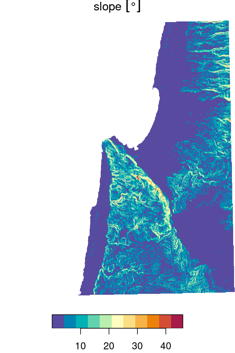
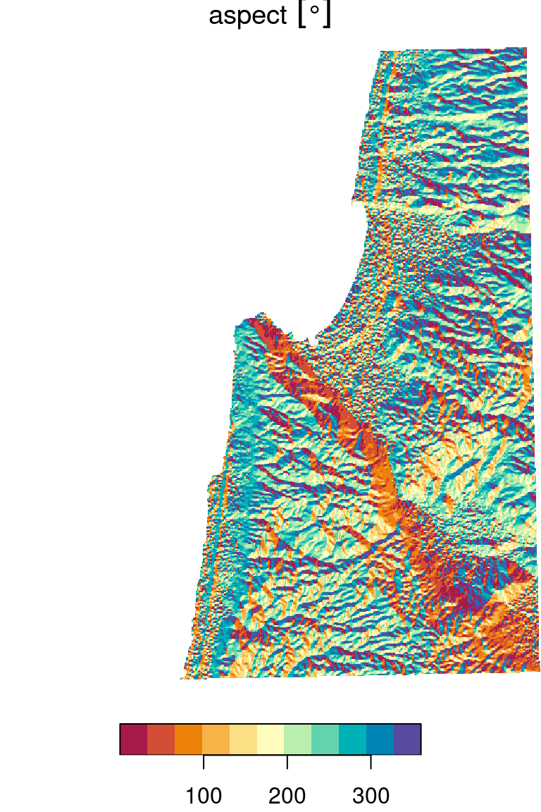
Figure 9.21: Topographic slope (left) and topographic aspect (right)
Note that our custom focal2+get_neighbors functions are quite minimal, and can be improved in several ways:
- Being able to set neighbor sizes other than \(3\times3\)
- Dealing with the first/last rows and and columns (see Section G)
- Dealing with rasters that have more than two dimensions (separate filter per dimension? a three-dimensional filter?)
- Making the calculation more efficient (e.g., using C/C++ code inside R or using parallel computation)