Chapter 3 Time series and function definitions
Last updated: 2021-03-31 00:23:36
Aims
Our aims in this chapter are:
- Working with data which represent time (dates)
- Learn how to visualize our data with graphical functions
- Learn to define custom functions
3.1 Dates
3.1.1 Date and time classes in R
In R, there are several special classes for representing times and time-series (time+data). For example:
- Times:
DatePOSIXctPOSIXlt
- Time series:
tszoo(packagezoo)xts(packagexts)
In this book, we will only be working with the Date class, which is used to represent times of type date.
3.1.2 Working with Date objects
3.1.2.1 Today’s date
The simplest data structure for representing times is Date, used to represent dates (without time of day). For example, we can get the current date with Sys.Date:
x = Sys.Date()
x
## [1] "2021-03-31"
Calling the class function (Section 1.3.11) on x reveals this is indeed an object of class Date:
class(x)
## [1] "Date"
3.1.2.2 Converting character to Date
We can also convert character values to Date, using as.Date. That way, we can create a Date object representing not just today’s date, but any date we want:
x = as.Date("2014-10-20")x
## [1] "2014-10-20"class(x)
## [1] "Date"When the character values are in the standard date format (YYYY-MM-DD), such as in the above example, the as.Date function works without any additional arguments. However, when the character values are in a non-standard format, we need to specify the format definition with format, using the various date component symbols. Table 3.1 lists the most commonly used symbols for specifying date formats in R. The full list of symbols can be found in ?strptime.
| Symbol | Example | Meaning |
|---|---|---|
%d |
"15" |
Day |
%m |
"08" |
Month, numeric |
%b |
"Aug" |
Month, 3-letter |
%B |
"August" |
Month, full |
%y |
14 |
Year, 2-digit |
%Y |
2014 |
Year, 4-digit |
Before going into examples of date formatting, it is useful to set the standard "C" locale in R. That way, we make sure that month or weekday names are interpreted in English as intended:
Sys.setlocale("LC_TIME", "C")
## [1] "C"
For example, converting the following character date—which is in a non-standard format—to Date fails when format is not specified:
as.Date("07/Aug/12")
## Error in charToDate(x): character string is not in a standard unambiguous format
Specifying the right format, which is "%d/%b/%y" in this case, leads to a successful conversion:
as.Date("07/Aug/12", format = "%d/%b/%y")
## [1] "2012-08-07"
What will be the result if we used
format="%y/%b/%d"(switching%dand%y) in the above expression?
Here is another example with a different non-standart format ("%Y-%B-%d"):
as.Date("2012-August-07")
## Error in charToDate(x): character string is not in a standard unambiguous formatas.Date("2012-August-07", format = "%Y-%B-%d")
## [1] "2012-08-07"3.1.2.3 Converting Date to character
A Date can always be converted back to character using as.character:
d = as.Date("1955-11-30")
d
## [1] "1955-11-30"class(d)
## [1] "Date"as.character(d)
## [1] "1955-11-30"class(as.character(d))
## [1] "character"Note that both the Date and the character objects are printed exactly the same way, so we have to use class to figure out which class we are dealing with.
The as.character function, by default, returns a text string with all three date components in the standard YYYY-MM-DD (or "%Y-%m-%d") format. Using the format argument, however, lets us compose different date formats, or extract individual date components out of a Date object:
d
## [1] "1955-11-30"as.character(d, format = "%m/%Y")
## [1] "11/1955"as.character(d, "%d")
## [1] "30"as.character(d, "%B")
## [1] "November"as.character(d, "%Y")
## [1] "1955"Note that as.character consistently returns a character, even when the result contains nothing but numbers, as in "%d" or "%Y". We can always convert from character to numeric with as.numeric if necessary:
as.numeric(as.character(d, "%Y"))
## [1] 1955
3.1.2.4 Arithmetic operations with dates
At this point, you may ask yourself why do we even bother to create Date objects, dealing with date formats, instead of simply working with character dates. The reason is that representing dates as Date makes it possible to do extremely useful operations, such as date arithmetic.
Date arithmetic means that Date objects act like numeric vectors, with respect to certain operations that make sense for dates, such as:
- Conditional operators—Comparing which date is earlier or later
- Subtraction—Calculating time differences
- Creating sequences with
seq—Creating date sequences
For example, the following expression uses a conditional operator to check whether today’s date is after 2013-01-01:
Sys.Date() > as.Date("2013-01-01")
## [1] TRUE
The subtraction operator (-) can be used to calculate the time difference between two dates. The result is an object of class difftime, which can be converted to numeric using as.numeric along with the unit we are interested in:
x = Sys.Date() - as.Date("2013-01-01")
x
## Time difference of 3011 daysas.numeric(x, unit = "hours")
## [1] 72264as.numeric(x, unit = "days")
## [1] 3011as.numeric(x, unit = "weeks")
## [1] 430.1429Finally, using the seq function—which we are already familiar with (Section 2.3.6.2)—we can create a sequence of consecutive dates. For example, the following expression creates a sequence of dates:
- starting at
"2018-10-14", - ending at (or before)
"2019-01-11", and - with a step size of 7 days
seq(from = as.Date("2018-10-14"), to = as.Date("2019-01-11"), by = 7)
##  [1] "2018-10-14" "2018-10-21" "2018-10-28" "2018-11-04" "2018-11-11"
##  [6] "2018-11-18" "2018-11-25" "2018-12-02" "2018-12-09" "2018-12-16"
## [11] "2018-12-23" "2018-12-30" "2019-01-06"
As you can see, Date is a vector-like class. Most of the methods we learned about vectors, such as subsetting or recycling, apply to Date objects exactly the same way as to numeric, character and logical vectors.
3.1.3 Time series
In this book, we will not be working with specialized time series classes, such as ts. Instead, we will use the straightforward “manual” approach of treating a sequence of measurements and a corresponding sequence of times when those measurements were taken as a time series. For example, let’s define two numeric vectors, water level in Lake Kinneret, in May and in November, in each year during 1991-2011:
may = c(
  -211.92,-208.80,-208.84,-209.12,-209.01,-209.60,-210.24,-210.46,-211.76,
  -211.92,-213.13,-213.18,-209.74,-208.92,-209.73,-210.68,-211.10,-212.18,
  -213.26,-212.65,-212.37
)
nov = c(
  -212.79,-209.52,-209.72,-210.94,-210.85,-211.40,-212.01,-212.25,-213.00,
  -213.71,-214.78,-214.34,-210.93,-210.69,-211.64,-212.03,-212.60,-214.23,
  -214.33,-213.89,-213.68
)
And the corresponding vector of measurement times, in this case—numeric values representing years:
year = 1991:2011
year
##  [1] 1991 1992 1993 1994 1995 1996 1997 1998 1999 2000 2001 2002 2003 2004 2005
## [16] 2006 2007 2008 2009 2010 2011
What was the average water level in May? in November?
Was the water level ever below -213 (the “red line”) in May? in November? We can find out using the any function (Section 2.4.1)11:
any(may < -213)
## [1] TRUEany(nov < -213)
## [1] TRUEHow can we find out in which year(s) was the water level below -213 in May? in November? We can use the logical vector nov < -213 to subset (Section 2.3.10.2) the year vector:
year[nov < -213]
## [1] 2000 2001 2002 2008 2009 2010 2011
year[may < -213]
## [1] 2001 2002 2009A table is more natural for representing a collection of corresponding vectors, such as the times and measurements that comprise a time series:
data.frame(year, may, nov)
##    year     may     nov
## 1  1991 -211.92 -212.79
## 2  1992 -208.80 -209.52
## 3  1993 -208.84 -209.72
## 4  1994 -209.12 -210.94
## 5  1995 -209.01 -210.85
## 6  1996 -209.60 -211.40
## 7  1997 -210.24 -212.01
## 8  1998 -210.46 -212.25
## 9  1999 -211.76 -213.00
## 10 2000 -211.92 -213.71
## 11 2001 -213.13 -214.78
## 12 2002 -213.18 -214.34
## 13 2003 -209.74 -210.93
## 14 2004 -208.92 -210.69
## 15 2005 -209.73 -211.64
## 16 2006 -210.68 -212.03
## 17 2007 -211.10 -212.60
## 18 2008 -212.18 -214.23
## 19 2009 -213.26 -214.33
## 20 2010 -212.65 -213.89
## 21 2011 -212.37 -213.68
We will learn about tables in Chapter 4.
3.2 Graphics
3.2.1 Generic functions
Some of the functions we learned about are generic functions. Generic functions are functions that can accept arguments of different classes. What the function does depends on the argument class, according to the method defined for that class. The advantages of having generic functions are easier remembering function names and ability to run the same code on different types of objects.
For example, print is a generic functions. When the print function gets a vector it prints the values, but when it gets a raster stars object its prints a summary of its properties (Section 1.1.5). Similarly, the graphical function plot (below) displays different graphical output depending on the type of input(s).
3.2.2 Graphical functions
The graphical function plot, given a numeric vector, displays its values in a two dimensional plot where:
- Vector indices are on the x-axis
- Vector values are on the y-axis
For example (Figure 3.1):
plot(nov, type = "b")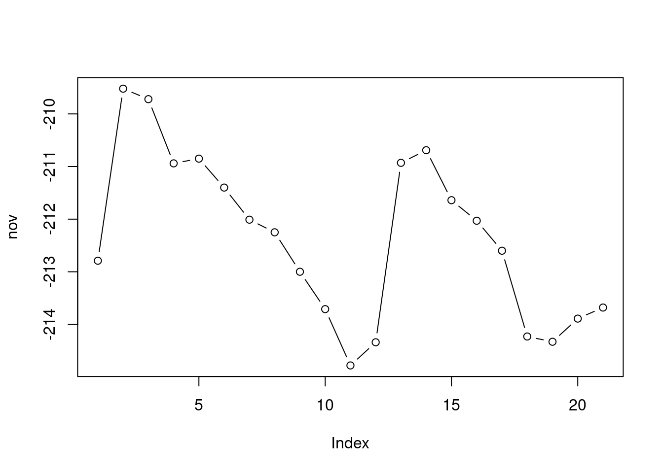
Figure 3.1: Plot of the nov vector
The type="b" argument means draw both points and lines. Other useful options for type include:
type="p"for points (the default)type="l"for linestype="o"for overplotted lines and points
If we pass two vectors to plot, the values of the first vector appears on the x-axis, while the values of the second vector appear on the y-axis. For example, we can put the years of water level measurement on the x-axis, as follows (Figure 3.2):
plot(year, nov, type = "b")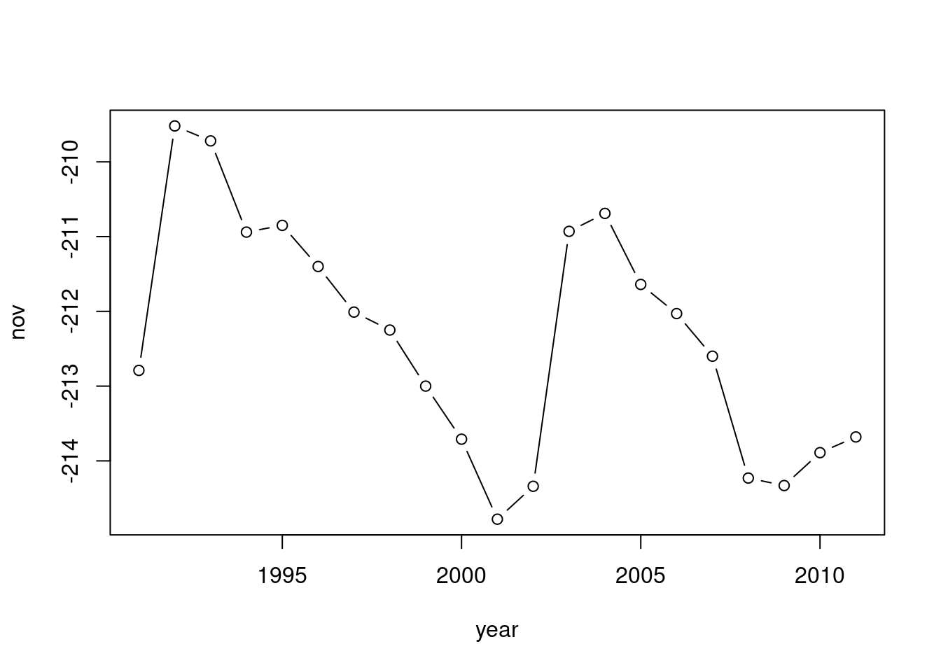
Figure 3.2: nov as function of year
We can add a horizontal line displaying the Kinneret “red line” using abline with the h parameter. The h parameter determines the y-axis value for the horizontal line. Note that abline draws an additional “layer” in an existing graphical device, which was initiated with plot (Figure 3.3):
plot(year, nov, type = "b")
abline(h = -213)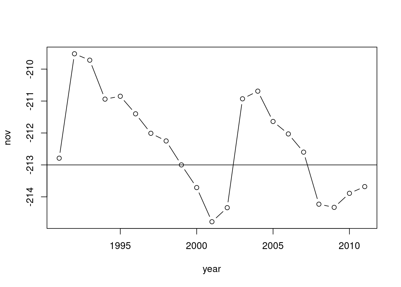
Figure 3.3: Adding a horizontal line with abline
Other additional “layers” can be added to an existing plot using the functions points and lines. For example, the following code section draws both the nov and may time series in the same plot. We are using the graphical parameter col to specify a different line color. In addition, we are setting the y-axis range with ylim to make sure both time series fit inside the displayed range. The ylim argument needs to be a vector of length two, the minimum and the maximum (Figure 3.4):
plot(year, nov, ylim = range(c(nov, may)), type = "b", col = "red")
lines(year, may, type = "b", col = "blue")
abline(h = -213)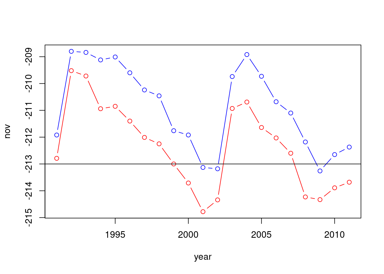
Figure 3.4: Adding a second series with lines
Finally, we can set the axis labels using the xlab and ylab parameters of the plot function (Figure 3.5):
plot(
  year, nov,
  xlab = "Year", ylab = "Elevation (m)",
  ylim = range(c(nov, may)),
  type = "b",
  col = "red"
)
lines(year, may, type = "b", col = "blue")
abline(h = -213)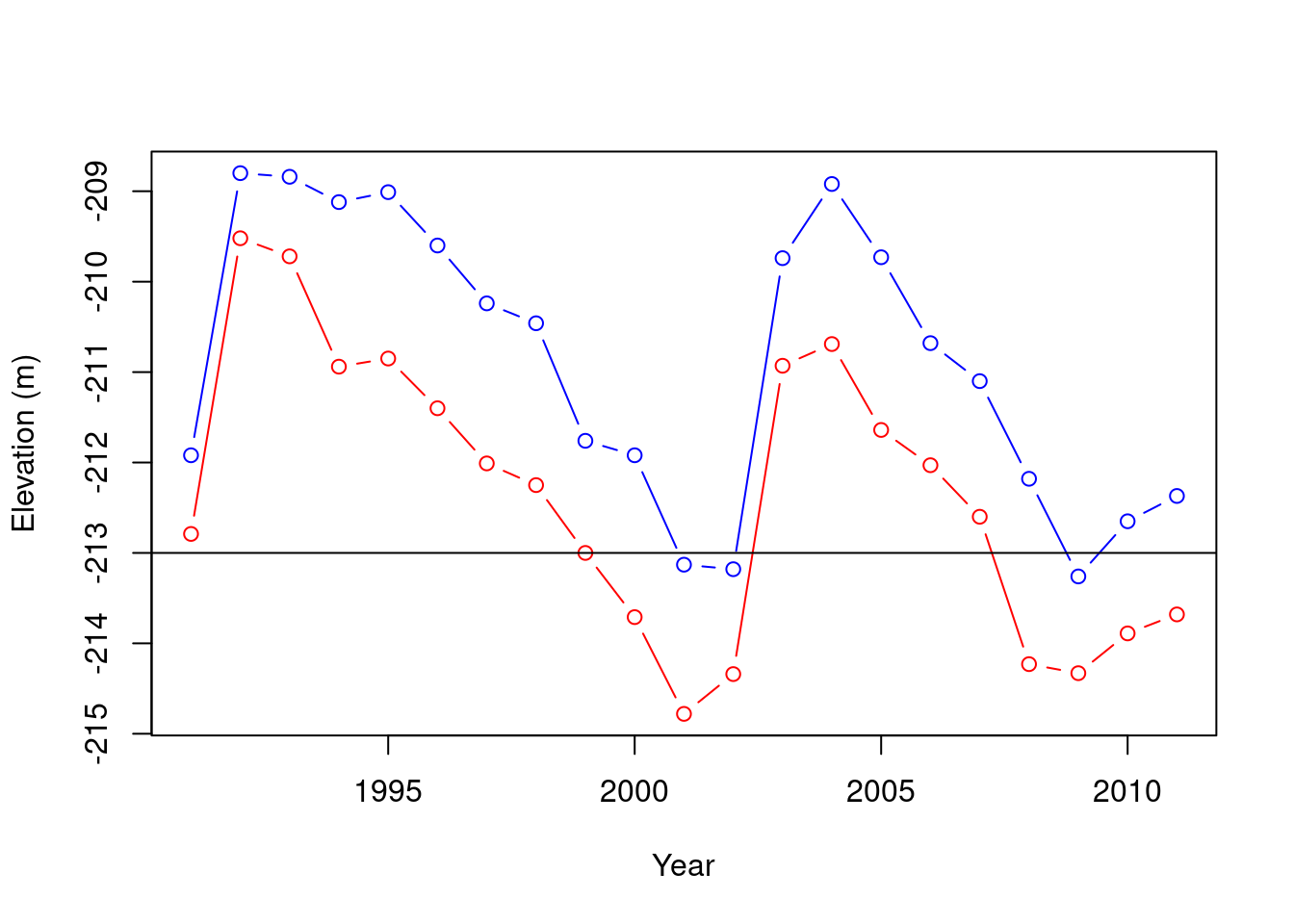
Figure 3.5: Setting axis labels
3.2.3 Consecutive differences
The diff function can be used to create a vector of differences between consecutive elements:
d_nov = c(NA, diff(nov))
d_nov
##  [1]    NA  3.27 -0.20 -1.22  0.09 -0.55 -0.61 -0.24 -0.75 -0.71 -1.07  0.44
## [13]  3.41  0.24 -0.95 -0.39 -0.57 -1.63 -0.10  0.44  0.21
Why do you think we added
NAat the beginning of the vector?
Now we can find out which year had the biggest water level increase or decrease:
year[which.max(d_nov)]  # Year of biggest increase
## [1] 2003
year[which.min(d_nov)]  # Year of biggest decrease
## [1] 2008
These results are visualized in Figure 3.6.
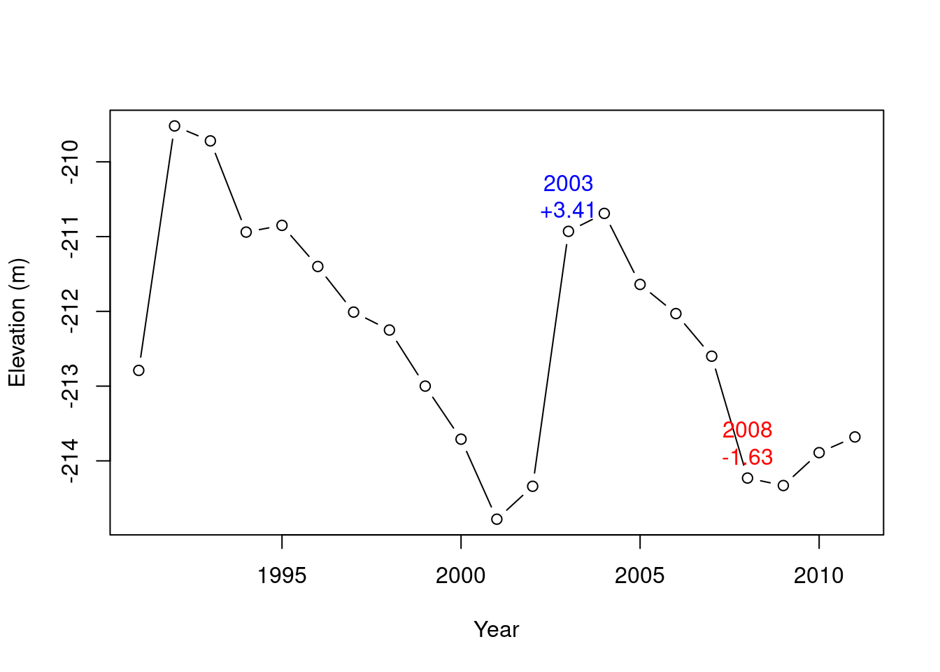
Figure 3.6: Years of biggest increase (2003) and decrease (2008) in the nov time series
Note that which.min and which.max ignore NA values.
3.3 Defining custom functions
3.3.1 Function definition components
In Section 1.3.6, we learned that a function call is an instruction to execute a certain function, as in:
f(arg1, arg2, ...)The function itself is actually an object containing code, which is loaded into the RAM, and can be executed with specific arguments. So far, we met functions defined in the default R packages (e.g., mean, seq, length, etc.). Later on we will also use functions from external packages 5.3.3. In this section, we learn how to define our own custom functions.
Here is the structure of a function definition expression in R:
add_five = function(x) {
  x_plus_five = x + 5
  return(x_plus_five)
}
The expression is composed of:
- A function name (
add_five) - The assignment operator (
=) - The function keyword (
function) - Parameter(s), inside parentheses and separated by commas (
(x)) - Curly brackets (
{) - Code (
x_plus_five = x + 5) - Returned value (
return(x_plus_five)) - Curly brackets (
})
3.3.2 Function definition vs. function call
The idea is that the code inside the function gets executed each time the function is called. For example, the function we just defines, add_five, can be used to calculate the sum of various numbers and five. Here is, again, the add_five function definition:
# Function definition
add_five = function(x) {
  x_plus_five = x + 5
  return(x_plus_five)
}
And here are two function calls of the add_five function, using different arguments 5 and 77:
# Function call, with argument 5
add_five(5)
## [1] 10
# Function call, with argument 77
add_five(77)
## [1] 82Note the returned values, 10 and 82, printed in the console.
3.3.3 Local variables
When we make a function call, the values we pass as function arguments are assigned to local variables which the function code can use. Those local variables are not accessible in the global environment. For example, even though we just executed two function calls of add_five, where the local variable x_plus_five was defined, x_plus_five is unavailable in the global environment:
x_plus_five
## Error in eval(expr, envir, enclos): object 'x_plus_five' not found
3.3.4 Returned value
Every function returns a value. We can assign the returned value to a variable, in case we want to keep it in memory for later use:
result = add_five(3)
result
## [1] 8
A return expression, such as the one we used in add_five, is optional and can be omitted:
return(x_plus_five)If the return expression is omitted, the returned value is the result of the last expression in the function body. The following alternative definition of add_five, where the assignment and the return expressions were omitted, is therefore identical:
add_five = function(x) {
  x + 5
}
We can also omit the { and } parentheses in case the code consists of a single expression. Therefore the add_five function definition can be simplified to much shorter code than our initial version, as follows:
add_five = function(x) x + 53.3.5 Default arguments
Default arguments (Section 2.3.7) can be specified as part of the function definition. In case there is a default value, we can skip that parameter in function calls.
For example, the following definition of add_five does not specify a default value for x. Therefore, trying to call add_five without passing an argument for x gives an error:
add_five = function(x) x + 5
add_five()
## Error in add_five(): argument "x" is missing, with no default
The following alternative definition does specify the default value of 1 for x. The default value is used when calling the function without specifying x:
add_five = function(x = 1) x + 5
add_five()
## [1] 6
3.3.6 Argument types
There are no restrictions for the classes and dimensions of arguments a function can accept, as long as we did not set such restrictions ourselves, e.g., using conditionals (Section 4.2.2). However, we get an error if one of the expressions in the function code is illegal given the arguments.
For example, the add_five function accepts vectors of length >1, adding five to each element:
add_five(1:3)
## [1] 6 7 8
However, passing a character value gives an error, because the internal expression x+5 cannot be executed:
add_five("one")
## Error in x + 5: non-numeric argument to binary operator
3.3.7 More examples
As another example, let’s define a function named last_minus_first which accepts a vector and returns the difference between the last and the first elements:
last_minus_first = function(x) {
  x[length(x)] - x[1]
}
Here are three different function calls to demontrate that our function indeed works as expected:
last_minus_first(1:3)
## [1] 2last_minus_first(nov)
## [1] -0.89last_minus_first(may)
## [1] -0.45Define a function named
modifythat accepts three arguments:
xindexvalueThe function assigns
valueinto the element at theindexposition of vectorx. The function returns the modified vectorx, as shown below.
modify(x = 1:10, index = 3, value = 55)
##  [1]  1  2 55  4  5  6  7  8  9 10
modify(x = 1:10, index = 9, value = NA)
##  [1]  1  2  3  4  5  6  7  8 NA 10
When typing
nov < -213, make sure there is a space between<and-. Otherwise the combination is interpreted as an assignment operator<-!↩︎