Chapter 6 Raster processing

Last updated: 2021-03-31 00:23:53

Aims

Our aims in this chapter are:

Learn how to get raster subsets
Learn to set raster dimension properties
Learn to calculate new rasters, based on one or more overlapping rasters, using raster algebra

We will use the following R packages:

stars

6.1 Time series for single pixel

6.1.1 Selecting pixel by row & column

In most of the examples in this chapter, we are going to use the MOD13A3_2000_2019.tif raster which we already met in Section 5.3. Let’s read it into memory:

library(stars)
r = read_stars("MOD13A3_2000_2019.tif")
names(r) = "NDVI"

Keep in mind this is a raster time series, where the “layers” refer to NDVI images taken in different times. As an exercise of accessing raster values (Section 5.3.8.4) and working with time series (Section 3.1.3), in this Section we are going to extract and plot a NDVI time series for a single pixel.

In Section 5.3.8.2, we saw how the matrix or array of raster values can be accessed using the [[ operator, as in r[[1]]. As another exercise, let’s access a “slice” of a single pixel through all of the raster layers, as follows:

v = r[[1]][50, 220, ]
class(v)
## [1] "numeric"

The result is a vector (why?). Plotting the vector displays a time-series of NDVI at a particular location (Figure 6.1):

plot(v, type = "o")

Figure 6.1: Single pixel values across all layers

6.1.2 Combining values with dates

The file MOD13A3_2000_2019_dates2.csv corresponds to the third dimension of MOD13A3_2000_2019.tif, containing the dates when each NDVI image was captured. This file includes the additional season column which we calculated in Section 4.6.

Using the MOD13A3_2000_2019_dates2.csv table, we can display dates on the x-axis (Figure 6.2). First we read the dates table:

dates = read.csv("MOD13A3_2000_2019_dates2.csv")
dates$date = as.Date(dates$date)

The we can plot the dates on the x-axis, as follows:

plot(dates$date, v, type = "o", xlab = "Time", ylab = "NDVI")

Figure 6.2: Single pixel values across all layers

6.1.3 Visualizing seasonal pattern

Figure 6.2 clearly shows the seasonal pattern of NDVI. However, we can further improve the interpretability of the time series plot if we mark seasons with different color. One way to do that is to plot the NDVI observations of each season one at a time, using a for loop.

As a first step, we define the vector of seasons (seasons) and the corresponding vector of colors (cols):

seasons = c("winter", "spring", "summer", "fall")
cols = c("blue", "purple", "red", "yellow")

Then, we can use a for loop (Section 4.2.3) to mark the portion of the NDVI time series from each season (Figure 6.3):

plot(dates$date, v, type = "l", xlab = "Time", ylab = "NDVI", col = "grey")
for(i in 1:length(seasons)) {
  tmp = v
  tmp[dates$season != seasons[i]] = NA
  lines(dates$date, tmp, col = cols[i], type = "o")
}

Figure 6.3: Single pixel values across all layers

6.2 Raster subsetting

6.2.1 Selecting rows, column and layers

We can get a subset of a stars object while keeping all of its properties, using the [ operator.

The stars subset operator [ works as follows:

The 1^st index selects attributes
The 2^nd index selects the first dimension, typically [x], i.e., raster columns
The 3^rd index selects the second dimension, typically [y], i.e., raster rows
The 4^th index selects the thirds dimension (if there is one), typically band, i.e., raster layers
(Subsequesnt indices, if any, select the remaining dimensions)

In this book, as well as in most spatial data analysis practices, we encounter two types of rasters: single-band rasters and multi-band rasters (Section 5.3.2). Accordingly, typical subsetting of stars objects requires either 3 or 4 indices. Again (Section 5.3.8.4), keep in mind that the order of stars indices is opposite of the order we are used to in R, since the first dimension refers to columns [x], while the second dimension refers to rows [y].

For example, the following expression creates a subset with two columns, three rows and four layers from r:

s = r[, 100:101, 200:202, 2:5]
s
## stars object with 3 dimensions and 1 attribute
## attribute(s):
##      NDVI        
##  Min.   :0.1575  
##  1st Qu.:0.1841  
##  Median :0.2261  
##  Mean   :0.2235  
##  3rd Qu.:0.2696  
##  Max.   :0.2852  
## dimension(s):
##      from  to  offset    delta  refsys point values x/y
## x     100 101 3239946  926.625 unnamed FALSE   NULL [x]
## y     200 202 3717158 -926.625 unnamed FALSE   NULL [y]
## band    2   5      NA       NA      NA    NA   NULL

The raster subset is plotted in Figure 6.4:

plot(round(s, 2), text_values = TRUE, col = terrain.colors(6), key.pos = 4)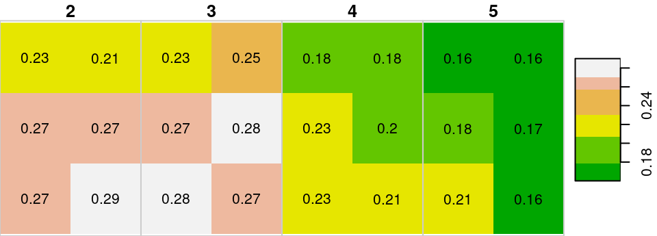

Figure 6.4: Raster subset with two columns, three rows and four layers

Note that we use the round function to round all raster values to two decimal places, so that the text labels can fit inside the pixels. This is an example of a raster algebra operation, which we learn about later in this chapter (Section 6.4).

What is the meaning of the following plot (Figure 6.5)?

plot(
  as.vector(r[,,,2][[1]]), 
  as.vector(r[,,,3][[1]]), 
  xlab = "Band 2", 
  ylab = "Band 3"
)

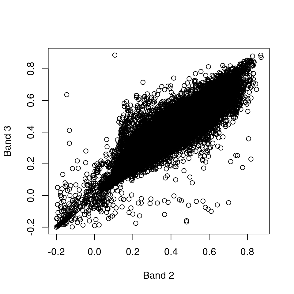
Figure 6.5: Band 3 as function of band 2

6.2.2 Dropping unnecessary dimensions

When a subset includes just one step along one or more dimensions, the “unnecessary” demensions can be dropped using drop=TRUE. For example, compare the output of the following two expressions. Both expressions return a subset consisting of the 7^th layer of r. However, the first expression returns a three-dimensional stars object (with a single layer in the 3^rd dimension), while the second expression returns a two-dimensional stars object where the 3^rd dimension was “dropped”:

r[,,,7]
## stars object with 3 dimensions and 1 attribute
## attribute(s):
##      NDVI        
##  Min.   :-0.199  
##  1st Qu.: 0.096  
##  Median : 0.112  
##  Mean   : 0.148  
##  3rd Qu.: 0.189  
##  Max.   : 0.852  
##  NA's   :9877    
## dimension(s):
##      from  to  offset    delta  refsys point values x/y
## x       1 167 3239946  926.625 unnamed FALSE   NULL [x]
## y       1 485 3717158 -926.625 unnamed FALSE   NULL [y]
## band    7   7      NA       NA      NA    NA   NULL

r[,,,7, drop = TRUE]
## stars object with 2 dimensions and 1 attribute
## attribute(s):
##      NDVI        
##  Min.   :-0.199  
##  1st Qu.: 0.096  
##  Median : 0.112  
##  Mean   : 0.148  
##  3rd Qu.: 0.189  
##  Max.   : 0.852  
##  NA's   :9877    
## dimension(s):
##   from  to  offset    delta  refsys point values x/y
## x    1 167 3239946  926.625 unnamed FALSE   NULL [x]
## y    1 485 3717158 -926.625 unnamed FALSE   NULL [y]

Accordingly, the raster values are represented as an array in the first case, and as a matrix in the second case:

class(r[,,,7][[1]])
## [1] "array"

class(r[,,,7, drop = TRUE][[1]])
## [1] "matrix" "array"

Note that the meaning of the drop parameter in stars subsetting differs from what we learned about in data.frame (Section 4.1.5.3) and matrix (Section 5.1.7.1) subsetting, in two respects. First, in stars subsetting drop=TRUE specifies dropping of raster dimensions, while in data.frame and matrix subsetting drop specifies simplifying to a different data structure (a vector). Second, the default of drop in stars is drop=FALSE, while in data.frame and matrix subsetting the default is drop=TRUE.

6.3 Raster dimensions

6.3.1 Getting dimension properties

As mentioned in Section 5.3.8.3, the st_dimensions function can be used to access dimension properties of a stars object. The function resurns an object of class dimensions. Printing the object gives all information on the raster dimensions in the form of a table:

st_dimensions(r)
##      from  to  offset    delta  refsys point values x/y
## x       1 167 3239946  926.625 unnamed FALSE   NULL [x]
## y       1 485 3717158 -926.625 unnamed FALSE   NULL [y]
## band    1 233      NA       NA      NA    NA   NULL

Internally, the dimensions object is a list of dimensions, with one list element per dimension. Each element is also a list, with the internal list elements being the various properties of a single dimension:

str(st_dimensions(r))
## List of 3
##  $ x   :List of 7
##   ..$ from  : num 1
##   ..$ to    : num 167
##   ..$ offset: num 3239946
##   ..$ delta : num 927
##   ..$ refsys:List of 2
##   .. ..$ input: chr "unnamed"
##   .. ..$ wkt  : chr "PROJCRS[\"unnamed\",\n    BASEGEOGCRS[\"unnamed ellipse\",\n        DATUM[\"unknown\",\n            ELLIPSOID[\"| __truncated__
##   .. ..- attr(*, "class")= chr "crs"
##   ..$ point : logi FALSE
##   ..$ values: NULL
##   ..- attr(*, "class")= chr "dimension"
##  $ y   :List of 7
##   ..$ from  : num 1
##   ..$ to    : num 485
##   ..$ offset: num 3717158
##   ..$ delta : num -927
##   ..$ refsys:List of 2
##   .. ..$ input: chr "unnamed"
##   .. ..$ wkt  : chr "PROJCRS[\"unnamed\",\n    BASEGEOGCRS[\"unnamed ellipse\",\n        DATUM[\"unknown\",\n            ELLIPSOID[\"| __truncated__
##   .. ..- attr(*, "class")= chr "crs"
##   ..$ point : logi FALSE
##   ..$ values: NULL
##   ..- attr(*, "class")= chr "dimension"
##  $ band:List of 7
##   ..$ from  : num 1
##   ..$ to    : int 233
##   ..$ offset: num NA
##   ..$ delta : num NA
##   ..$ refsys: chr NA
##   ..$ point : logi NA
##   ..$ values: NULL
##   ..- attr(*, "class")= chr "dimension"
##  - attr(*, "raster")=List of 3
##   ..$ affine     : num [1:2] 0 0
##   ..$ dimensions : chr [1:2] "x" "y"
##   ..$ curvilinear: logi FALSE
##   ..- attr(*, "class")= chr "stars_raster"
##  - attr(*, "class")= chr "dimensions"

Individual dimensions can be accessed using the $ operator by list element name, or the [[ operator by list element index or name (more on lists in Section 11.1). For example, all three expressions shown below return the same result, the properties of the 1^st dimension "x":

str(st_dimensions(r)[[1]])
## List of 7
##  $ from  : num 1
##  $ to    : num 167
##  $ offset: num 3239946
##  $ delta : num 927
##  $ refsys:List of 2
##   ..$ input: chr "unnamed"
##   ..$ wkt  : chr "PROJCRS[\"unnamed\",\n    BASEGEOGCRS[\"unnamed ellipse\",\n        DATUM[\"unknown\",\n            ELLIPSOID[\"| __truncated__
##   ..- attr(*, "class")= chr "crs"
##  $ point : logi FALSE
##  $ values: NULL
##  - attr(*, "class")= chr "dimension"

str(st_dimensions(r)[["x"]])
## List of 7
##  $ from  : num 1
##  $ to    : num 167
##  $ offset: num 3239946
##  $ delta : num 927
##  $ refsys:List of 2
##   ..$ input: chr "unnamed"
##   ..$ wkt  : chr "PROJCRS[\"unnamed\",\n    BASEGEOGCRS[\"unnamed ellipse\",\n        DATUM[\"unknown\",\n            ELLIPSOID[\"| __truncated__
##   ..- attr(*, "class")= chr "crs"
##  $ point : logi FALSE
##  $ values: NULL
##  - attr(*, "class")= chr "dimension"

str(st_dimensions(r)$x)
## List of 7
##  $ from  : num 1
##  $ to    : num 167
##  $ offset: num 3239946
##  $ delta : num 927
##  $ refsys:List of 2
##   ..$ input: chr "unnamed"
##   ..$ wkt  : chr "PROJCRS[\"unnamed\",\n    BASEGEOGCRS[\"unnamed ellipse\",\n        DATUM[\"unknown\",\n            ELLIPSOID[\"| __truncated__
##   ..- attr(*, "class")= chr "crs"
##  $ point : logi FALSE
##  $ values: NULL
##  - attr(*, "class")= chr "dimension"

Properties of individual dimensions can be accessed through further subsetting (Figure 6.6). For example, the following expression returns the offset and delta (resolution) properties of the "x" dimension:

st_dimensions(r)$x$delta
## [1] 926.6254

st_dimensions(r)$x$offset
## [1] 3239946

Figure 6.6: The hierarchical structure of stars dimensions properties

The meanings of the seven properties that every stars dimension has are summarized in Table 6.1.

Table 6.1: Dimension properties in a `stars` object
Property	Contents	Description
`from`	`numeric` length 1	The start index
`to`	`numeric` length 1	The end index
`offset`	`numeric` length 1	The start coordinate (or time) of the first element (e.g., the pixel/cell boundary)
`delta`	`numeric` length 1	The increment / cell size (e.g., the resolution)
`refsys`	`character`, or `crs`	The Coordinate Reference System (e.g., the CRS)
`point`	`logical` length 1	Whether cells/pixels refer to areas/periods (`FALSE`), or to points/instances (`TRUE`)
`values`	`NULL`, or an object that gives the specific dimension values	The dimension values, in case they are not calculated from `offset` and `delta`

For more information on stars dimensions, see the official stars Data Model article.

6.3.2 Setting dimension properties

A .tif file cannot hold metadata regarding raster “layers,” such as the date when the images were captured in case the layers comprise a time series, or the band names in case the layers comprise spectral bands (Section 6.4.2). Accordingly, the third dimension of a stars object created from GeoTIFF file does not contain any information other than the from and to indices (e.g., 1 and 233):

st_dimensions(r)
##      from  to  offset    delta  refsys point values x/y
## x       1 167 3239946  926.625 unnamed FALSE   NULL [x]
## y       1 485 3717158 -926.625 unnamed FALSE   NULL [y]
## band    1 233      NA       NA      NA    NA   NULL

We can incorporate more information into a stars object dimensions, or modify the existing information, on our own. This is done using function st_set_dimensions, where we need to specify:

.x—The stars object
which—The index (e.g., 1) or name (e.g., "x") of the dimension to be modified

as well as the dimension properties and their new values, such as:

offset—The offset
delta—The delta (i.e., resolution)
values—The values along the dimension
names—The new dimension names

as in st_set_dimensions(r, "x", offset = 0, delta = 1000).

Additionally, the names of all dimensions can be modified using (i.e., without specifying which):

.x— The stars object
names—The new dimension names

as in st_set_dimensions(r, names = c("a", "b", "c")).

For example, for a non-spatial dimension that represents time, such as the "band" dimension in r, we can set the values (the dates or times) as follows:

r = st_set_dimensions(r, "band", values = dates$date)

and the dimension names, as follows:

r = st_set_dimensions(r, names = c("x", "y", "time"))

Now, the 3^rd dimension of r is named "time" and contains the Date values:

st_dimensions(r)
##      from  to  offset    delta  refsys point                    values x/y
## x       1 167 3239946  926.625 unnamed FALSE                      NULL [x]
## y       1 485 3717158 -926.625 unnamed FALSE                      NULL [y]
## time    1 233      NA       NA    Date    NA 2000-02-01,...,2019-06-01

If necessary, the dimension values can be read back using st_get_dimension_values. For example:

z = st_get_dimension_values(r, "time")
class(z)
## [1] "Date"
z[1:10]
##  [1] "2000-02-01" "2000-03-01" "2000-04-01" "2000-05-01" "2000-06-01"
##  [6] "2000-07-01" "2000-08-01" "2000-09-01" "2000-10-01" "2000-11-01"

What is the meaning of the dimension values given by st_get_dimension_values(r, "x") and st_get_dimension_values(r, "y")? Given that st_dimensions(r)$y$values and st_dimensions(r)$y$values are NULL, where do you think these dimension values come from?

Why do we need to bother with editing or supplementing dimension properties? One reason is that it is more convenient to have all of the relevant raster data in the same object (rather than two separate objects, such as r and dates). Moreover, information regarding stars dimensions is utilized by stars functions in various contexts. For example, the layer values apprear as labels in plot output panels (Figure 6.7):

plot(r[,,,1:5], breaks = "equal", col = hcl.colors(11, "Spectral"), key.pos = 4)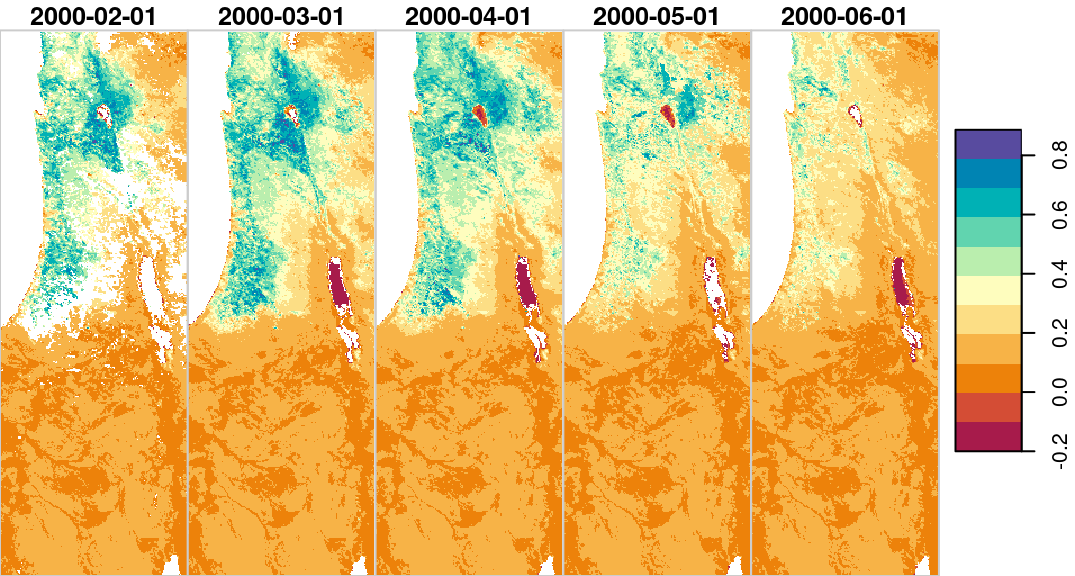

Figure 6.7: Date lables for raster layers, i.e., the third raster dimension

or as column values when converting from stars to data.frame:

head(as.data.frame(r))
##         x       y       time NDVI
## 1 3240409 3716695 2000-02-01   NA
## 2 3241336 3716695 2000-02-01   NA
## 3 3242262 3716695 2000-02-01   NA
## 4 3243189 3716695 2000-02-01   NA
## 5 3244116 3716695 2000-02-01   NA
## 6 3245042 3716695 2000-02-01   NA

6.3.3 Converting a `matrix` to raster

6.3.3.1 The `volcano` matrix

Converting a matrix to a stars raster is rarely needed in practice, since most of the time you will be working with existing rasters imported from files (Section 5.3.2). However, experimenting with the matrix→stars conversion will help us better understand the nature of rasters, in general, and of the stars class, in particular.

When converting a matrix or an array to a stars raster, we must manually set the properties of the dimensions, most importantly the spatial dimensions "x" and "y".

In the first example, we will convert the built-in volcano matrix (Section 5.1.6) to a stars raster. First, we convert the transposed (why? see Section 5.3.8.4) matrix to a stars raster, using function st_as_stars:

v = st_as_stars(t(volcano))
v
## stars object with 2 dimensions and 1 attribute
## attribute(s):
##       A1        
##  Min.   : 94.0  
##  1st Qu.:108.0  
##  Median :124.0  
##  Mean   :130.2  
##  3rd Qu.:150.0  
##  Max.   :195.0  
## dimension(s):
##    from to offset delta refsys point values x/y
## X1    1 61      0     1     NA FALSE   NULL [x]
## X2    1 87      0     1     NA FALSE   NULL [y]

Then, we may want to set the dimension and attribute names:

v = st_set_dimensions(v, names = c("x", "y"))
names(v) = "elevation"
v
## stars object with 2 dimensions and 1 attribute
## attribute(s):
##    elevation    
##  Min.   : 94.0  
##  1st Qu.:108.0  
##  Median :124.0  
##  Mean   :130.2  
##  3rd Qu.:150.0  
##  Max.   :195.0  
## dimension(s):
##   from to offset delta refsys point values x/y
## x    1 61      0     1     NA FALSE   NULL [x]
## y    1 87      0     1     NA FALSE   NULL [y]

Finally, we set the offset and delta of the x and y dimensions, or, other words, where do these axes start from and what is their step size (i.e., resolution). The offset values of 0 (see below), in this case, is arbitrary. The delta is also arbitrary, but should be equal for both "x" and "y" dimensions (unless we want to have asymmetrical pixels). In this case, according to the ?volcano help page, the matrix represents a 10m by 10m grid. Accordingly, we use delta values of 10 and -10 so that the coordinate units are “meters.” The delta of the y-axis is negative (!), so that the the values decrease when going to from 1^st row to last:

v = st_set_dimensions(v, "x", offset = 0, delta = 10)
v = st_set_dimensions(v, "y", offset = 0, delta = -10)
v
## stars object with 2 dimensions and 1 attribute
## attribute(s):
##    elevation    
##  Min.   : 94.0  
##  1st Qu.:108.0  
##  Median :124.0  
##  Mean   :130.2  
##  3rd Qu.:150.0  
##  Max.   :195.0  
## dimension(s):
##   from to offset delta refsys point values x/y
## x    1 61      0    10     NA    NA   NULL [x]
## y    1 87      0   -10     NA    NA   NULL [y]

Compare the output of plot(v, axes=TRUE) before and after setting the offset and delta to see the effect of those settings.

The result is shown in Figure 6.8. Note that we need to use the reset=FALSE argument whenever we want to have additional layers, such as a contours, in a stars plot:

plot(v, axes = TRUE, breaks = "equal", col = terrain.colors(100), key.pos = 4, reset = FALSE)
contour(v, add = TRUE)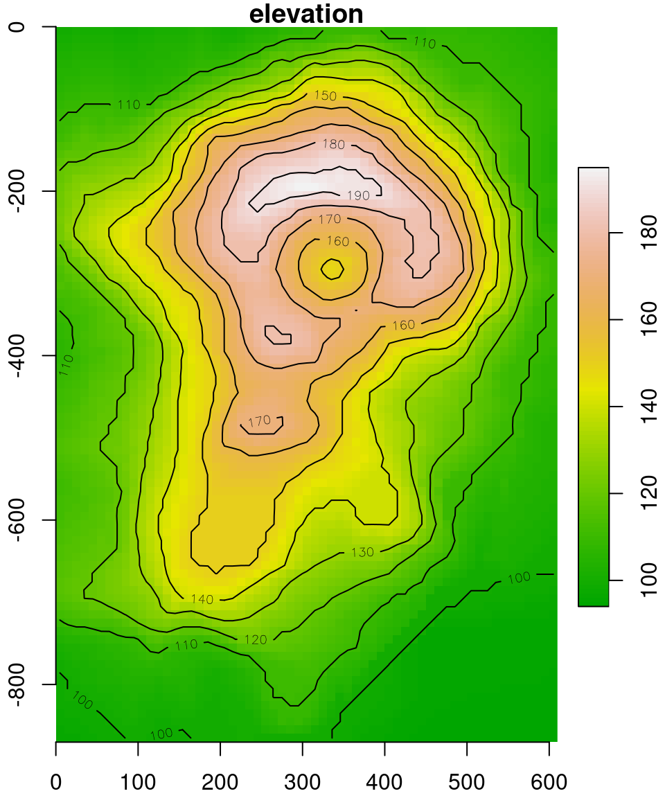

Figure 6.8: The volcano matrix converted to stars raster

The fact that the offset is arbitrary is demonstrated with the following expression, which “shifts” the raster so that the (0, 0) coordinate is in the botton-left rather than top-left corner:

v = st_set_dimensions(v, "y", offset = ncol(v) * 10, delta = -10)

The modified volcano raster is shown in Figure 6.9.

plot(v, axes = TRUE, breaks = "equal", col = terrain.colors(100), key.pos = 4, reset = FALSE)
contour(v, add = TRUE)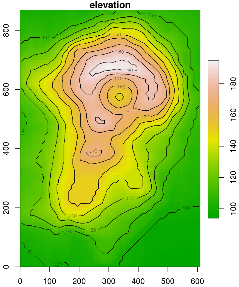

Figure 6.9: The volcano raster with modified offset

Comparing Figures 6.8 and 6.9, the only thing that has changed are the y-axis coordinates.

6.3.3.2 The Haifa DEM matrix

In the second example, we will recreate the dem.tif small DEM of Haifa using a matrix with its values. Here is the matrix we start with:

v = c(
  NA, NA, NA, NA, NA, NA, NA, 3, 5, 7, 
  NA, NA, NA, 61, 106, 47, 31, 39, 32, 49, 
  NA, NA, NA, 9, 132, 254, 233, 253, 199, 179, 
  NA, NA, NA, 4, 11, 146, 340, 383, 357, 307, 
  NA, 4, 6, 9, 6, 6, 163, 448, 414, 403, 
  3, 6, 9, 10, 6, 6, 13, 152, 360, 370, 
  3, 4, 7, 16, 27, 12, 64, 39, 48, 55
)
m = matrix(v, nrow = 10, ncol = 7)
m
##       [,1] [,2] [,3] [,4] [,5] [,6] [,7]
##  [1,]   NA   NA   NA   NA   NA    3    3
##  [2,]   NA   NA   NA   NA    4    6    4
##  [3,]   NA   NA   NA   NA    6    9    7
##  [4,]   NA   61    9    4    9   10   16
##  [5,]   NA  106  132   11    6    6   27
##  [6,]   NA   47  254  146    6    6   12
##  [7,]   NA   31  233  340  163   13   64
##  [8,]    3   39  253  383  448  152   39
##  [9,]    5   32  199  357  414  360   48
## [10,]    7   49  179  307  403  370   55

This time, assuming we know the right spatial reference information, we can create a truly georeferenced stars object. To position a matrix or array in geographic space (Section 5.3.1), we need to know the coordinates of the starting point (offset) and the resolution (delta) for the "x" and "y" dimensions. We also need to know the CRS that the offset and delta refer to.

For example, the following code section sets the two offset values (679624 and 3644759), the resolution (2880) and the CRS (32636). Note that the CRS is specified using st_set_crs and an EPSG code. In this case, the EPSG code 32636 specifies the CRS named “UTM zone 36N.” Again, the y-axis resolution is negative, so that going down the matrix rows translates to decreasing y-axis values.

s = st_as_stars(t(m))
s = st_set_dimensions(s, names = c("x", "y"))
s = st_set_dimensions(s, "x", offset = 679624, delta = 2880)
s = st_set_dimensions(s, "y", offset = 3644759, delta = -2880)
s = st_set_crs(s, 32636)
names(s) = "elevation"

The result is identical to dem.tif (Figure 5.14), as shown in Figure 6.10:

plot(s, text_values = TRUE, axes = TRUE, breaks = "equal", col = terrain.colors(10), key.pos = 4)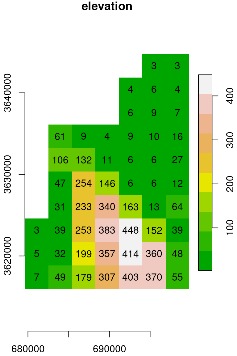

Figure 6.10: matrix converted to a stars object: Digital Elevation Model (DEM) of haifa

The effect of transposing the input matrix and modifying the sign of the y-axis delta is summarized in Figure 6.11. As we can see from this image, when delta_y is negative (while delta_x is positive), a transposed raster layer matrix, i.e., t(r[[1]]), matches the “true” spatial arrangement of the raster values. This is the most common scenario and the only one we will encounter in this book.

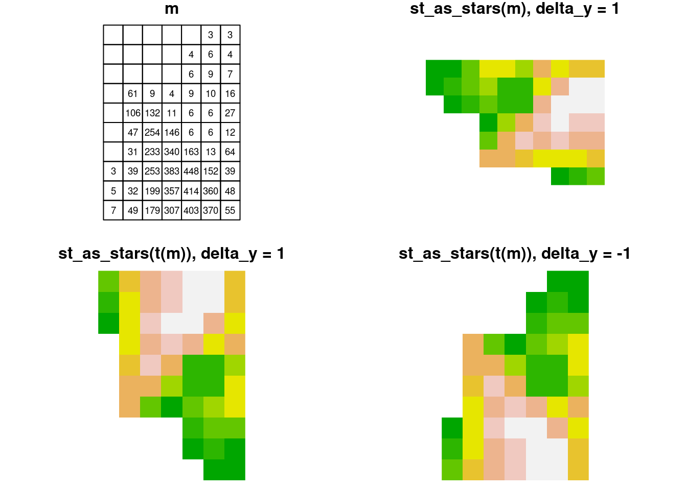
Figure 6.11: Converting matrix to stars: the effect of transposing the input matrix and modifying the sign of the y-axis delta

6.4 Raster algebra

6.4.1 Arithmetic and logical operations on layers

Raster algebra is the application of functions on a cell-by-cell basis, repeatedly for all pixels of one or more overlapping rasters. For example, we can apply the + (or sum) function on two overlapping rasters to obtain a new raster, where each pixel value is the sum of the corresponding pixel values from the two inputs (Figure 6.12).

Figure 6.12: Raster algebra (http://rpubs.com/etiennebr/visualraster)

Similarly, we can use any arithmetic (Section 1.3.2) or conditional (Section 1.3.4) operator:

Arithmetic: +, -, *, /
Logical: <, <=, >, >=, ==, !=, !

to make calculations on each pair of overlapping rasters, to get a new raster where each pixel value is the result of the given operation on the overlapping pixels in the input rasters. The operations can also combine rasters and numeric values, in which case the numeric value is recycled, as in r>5.

We can also use functions such as:

Functions: abs, round, ceiling, floor, sqrt, log, log10, exp, cos, sin

which are applied on an individual raster, transforming each of its pixels, separately.

For the next few examples, let’s create two single-band rasters named x and y. Note that we are using round to transform each of the rasters to rounded values with two decimal places (so that it is more convenient to display text labels):

x = r[, 99:101, 202:204, 1, drop = TRUE]
y = r[, 99:101, 200:202, 2, drop = TRUE]
x = round(x, 2)
y = round(y, 2)

Figure 6.13 shows the two rasters x and y:

plot(x, text_values = TRUE, main = "x", col = terrain.colors(5))
plot(y, text_values = TRUE, main = "y", col = terrain.colors(6))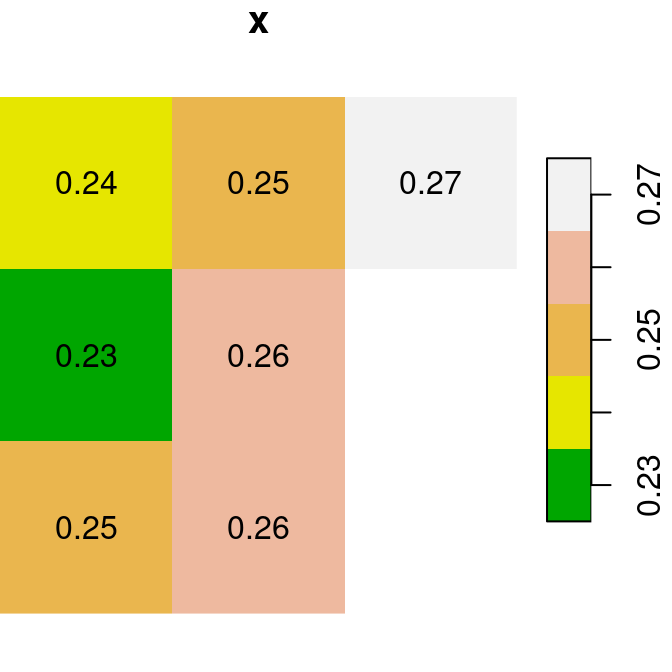

Figure 6.13: Two small stars rasters x and y to demonstrate raster algebra

As a first example of raster algebra, we calculate x+y, where each pixel value is the sum of two corresponding pixels in x and y (Figure 6.14):

plot(x, text_values = TRUE, main = "x", col = terrain.colors(5))
plot(y, text_values = TRUE, main = "y", col = terrain.colors(6))
plot(x + y, text_values = TRUE, main = "x+y", col = terrain.colors(5))

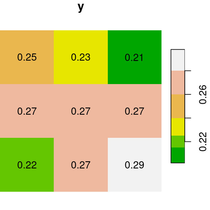
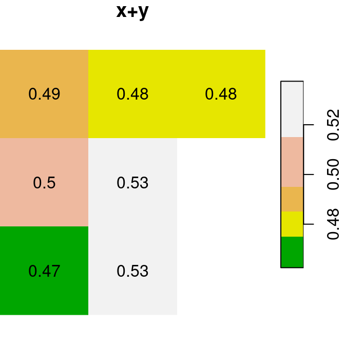
Figure 6.14: x, y and x+y

Why are two pixels in the bottom-right of x+y in Figure 6.14 displayed without any labels?

Here are several other examples of raster algebra: x-y, x*y and x+5. Note that x+5 combines a raster and a numeric value, rather than two rasters, in which case the numeric value is recycled (Figure 6.15):

plot(x - y, text_values = TRUE, main = "x-y", col = terrain.colors(5))
plot(x * y, text_values = TRUE, main = "x*y", col = terrain.colors(6))
plot(x + 5, text_values = TRUE, main = "x+5", col = terrain.colors(5))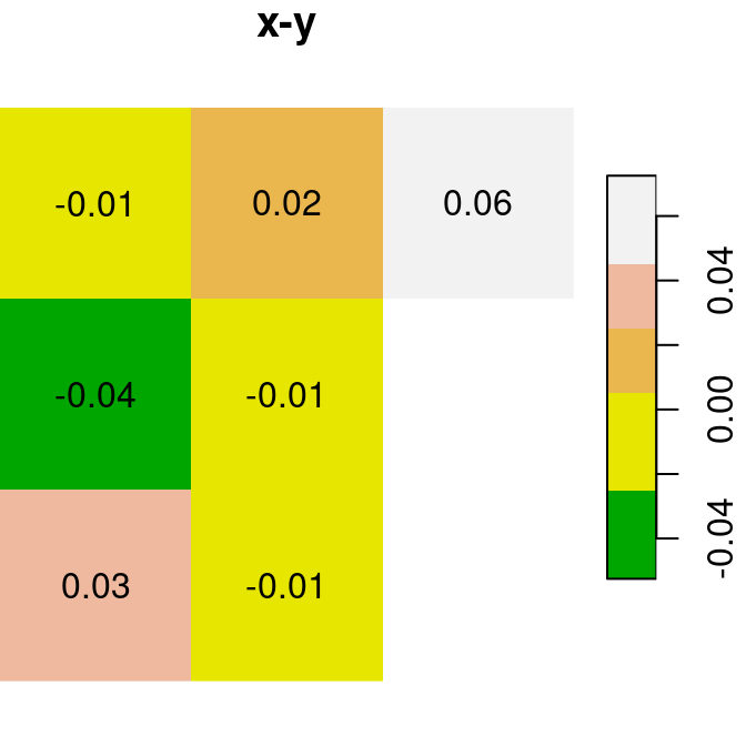

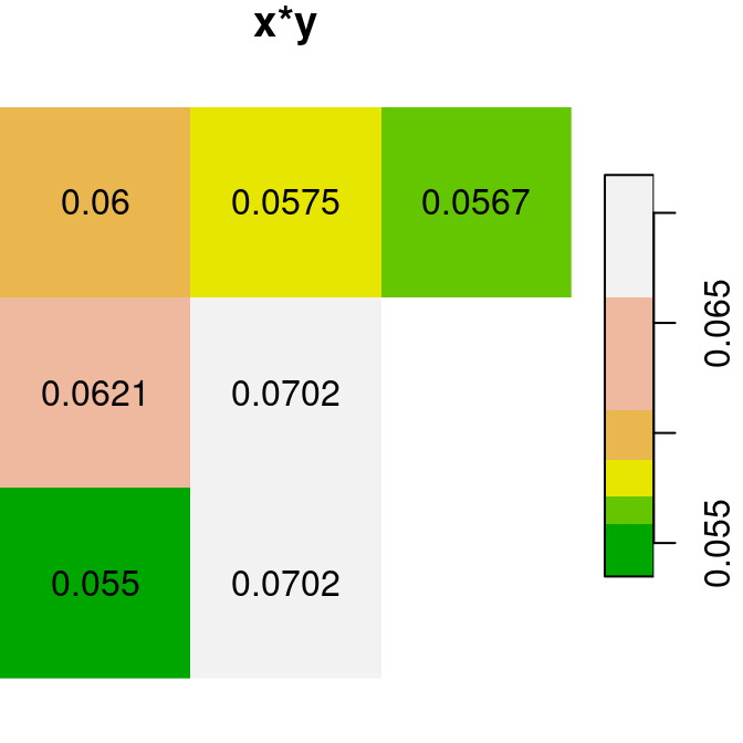
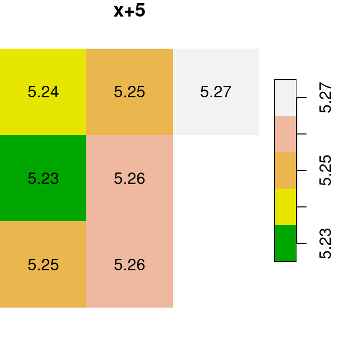
Figure 6.15: x, y and x+y

A logical raster algebra operation produces a logical raster, a raster where pixel values are TRUE or FALSE (or NA). For example, Figure 6.16 shows the logical rasters x>0.25, x<y and is.na(x):

plot(x > 0.25, text_values = TRUE, main = "x>0.25", col = terrain.colors(2, rev = TRUE))
plot(x < y, text_values = TRUE, main = "x<y", col = terrain.colors(2, rev = TRUE))
plot(is.na(x), text_values = TRUE, main = "is.na(x)", col = terrain.colors(2, rev = TRUE))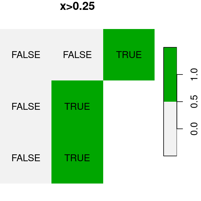

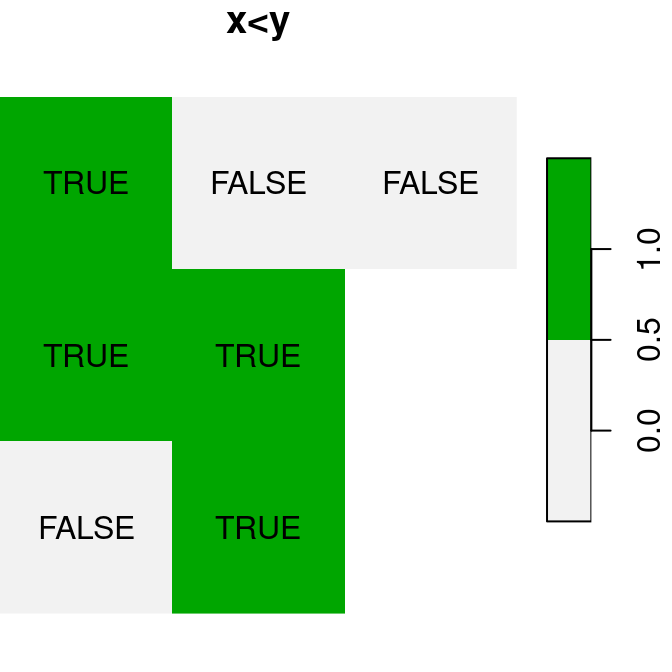
Logical raster algebra operations: `x>0.25`, `x<y` and `is.na(x)`

Figure 6.16: Logical raster algebra operations: x>0.25, x<y and is.na(x)

The last three examples produce logical rasters (Figure 6.16), which we have not encountered so far. In operations where a numeric representation is required, such as:

An arithmetic operation
Saving to a file

logical raster values TRUE and FALSE automatically become 1 and 0, respectively, similarly to what happens with vectors (Section 2.3.10.1). For example (Figure 6.17):

plot(is.na(x), text_values = TRUE, main = "is.na(x)", col = terrain.colors(2, rev = TRUE))
plot(is.na(x) * 1, text_values = TRUE, main = "is.na(x)*1", col = terrain.colors(2, rev = TRUE))
plot(is.na(x) + 30, text_values = TRUE, main = "is.na(x)+30", col = terrain.colors(2, rev = TRUE))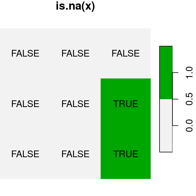

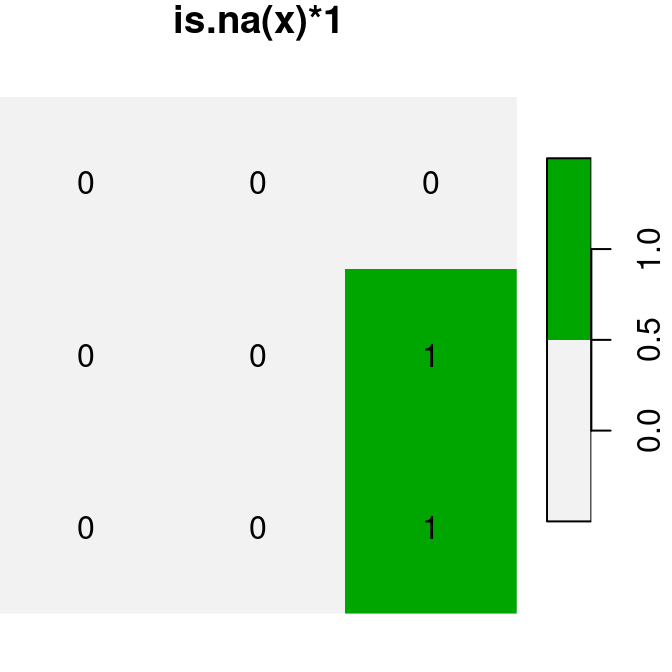
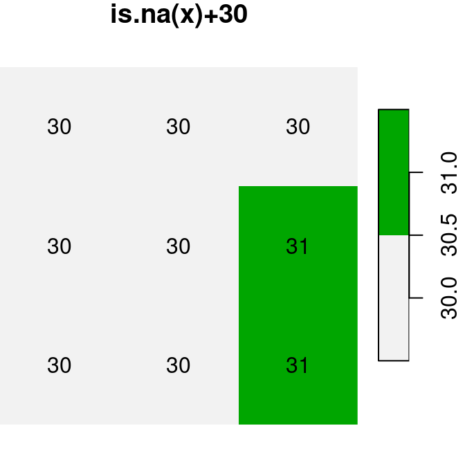
Conversion of raster values from `logical` to `numeric`

Figure 6.17: Conversion of raster values from logical to numeric

A logical raster can be used to assign new values into a subset of raster values. For example, we can use the logical raster is.na(x) to replace all NA values in the raster x with a new value:

x1 = x
x1[is.na(x1)] = 0.21

The “before” and “after” images are shown in Figure 6.18:

plot(x, text_values = TRUE, breaks = seq(0.2, 0.3, 0.02), col = terrain.colors(5), main = "Before")
plot(x1, text_values = TRUE, breaks = seq(0.2, 0.3, 0.02), col = terrain.colors(5), main = "After")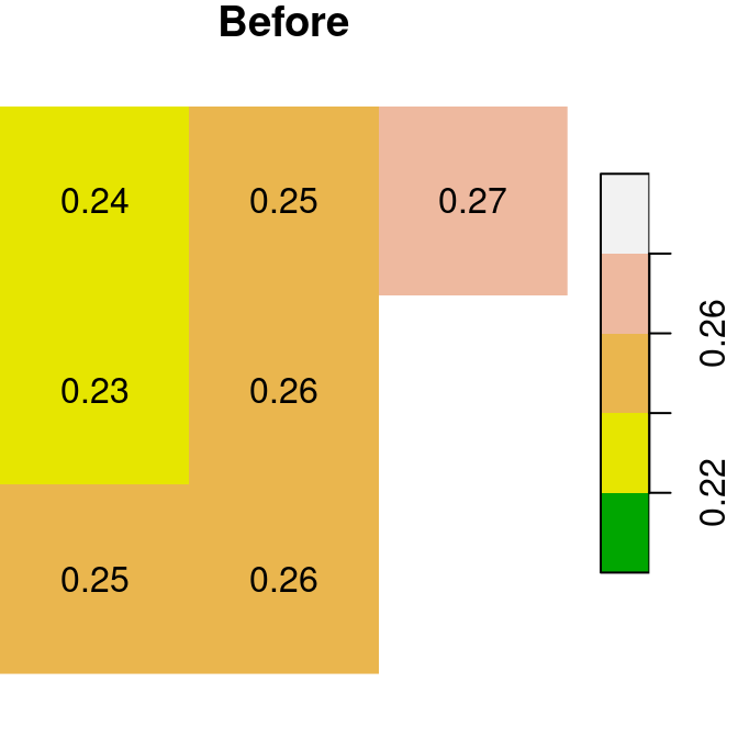

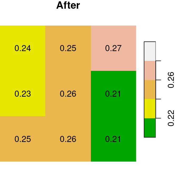
Figure 6.18: Assignmnent to raster subset using logical raster (before and after)

How can we replace the NA values in x with the average of all non-missing values?

How can we calculate the proportion of NA values in x?

6.4.2 Landsat image

For the following example, let’s read another multi-band raster file named landsat_04_10_2000.tif. This is a part of a Landsat-5 satellite image with bands 1-5 and 7, after radiometric and atmospheric corrections. The raster values represent spectral reflectance, therefore all values are between 0 and 1.

l = read_stars("landsat_04_10_2000.tif")

We can assign meaningful layer names according to the spectral range that is captured by each band²³:

bands = c("Blue", "Green", "Red", "NIR", "SWIR1", "SWIR2")
l = st_set_dimensions(l, "band", values = bands)
names(l) = "reflectance"

Protting the raster shows the reflectance images for each spectral band (Figure 6.19):

plot(l, breaks = "equal", key.pos = 4)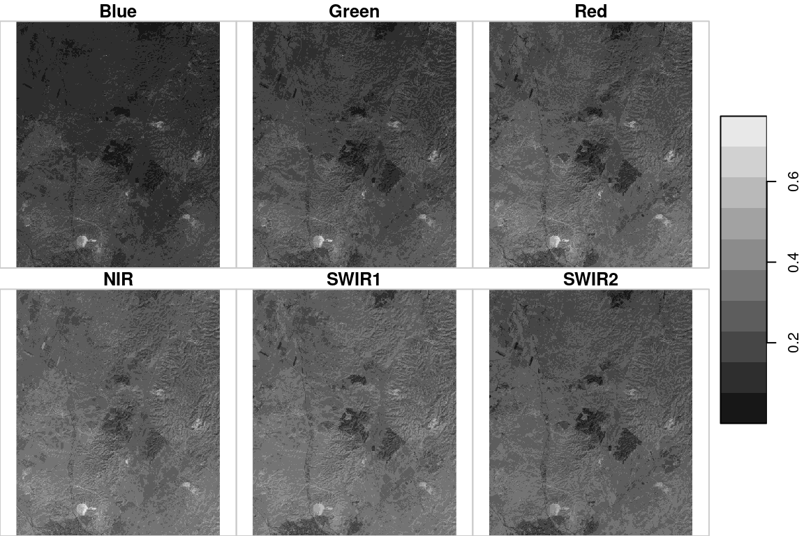

Figure 6.19: Landsat satellite image, bands 1-5 and 7

6.4.3 True color and false color images

An RGB image is an image where the colors are defines based on red, green, and blue intensity per pixel. An RGB image can therefore be constructed from red, green, and blue bands in a multispectral sensor (Figure 6.20), such as the ones in a digital camera or a satellite.

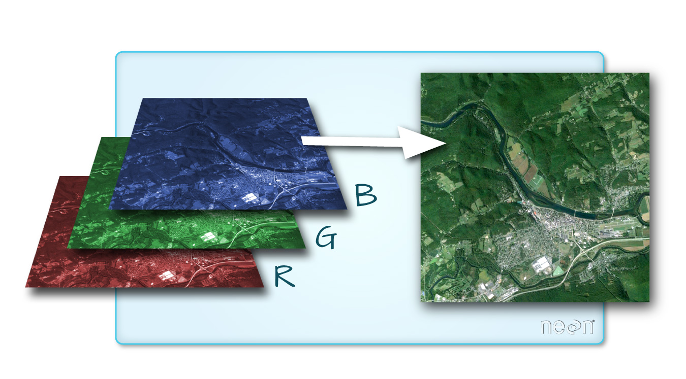
Figure 6.20: RGB image (https://datacarpentry.org/organization-geospatial/01-spatial-data-structures-formats/index.html)

A true color image is an image where the red, green and blue reflectance are red, green and blue colors. A true color image thus simulates the way that we would see the photographed area when looking from above, with the human eye. A false color image is an image where colors are mapped in any different way. A false color image can also include spectral bands that the human eye connot see, such as Near Infra Red (NIR).

True color and false color images can be produced with the plot function, specifying the red, green and blue bands with the rgb parameter. For example, in the Landsat image l, red, green and blue bands are 3, 2 and 1, therefore specifying rgb=c(3,2,1) produces a true color image (Figure 6.21). A different designation, rgb=c(4,3,2), produces a commonly used false color image where NIR is mapped to red, red is mapped to green and green is mapped to blue²⁴ (Figure 6.21):

plot(l, rgb = c(3, 2, 1), main = "True color")
plot(l, rgb = c(4, 3, 2), main = "False color")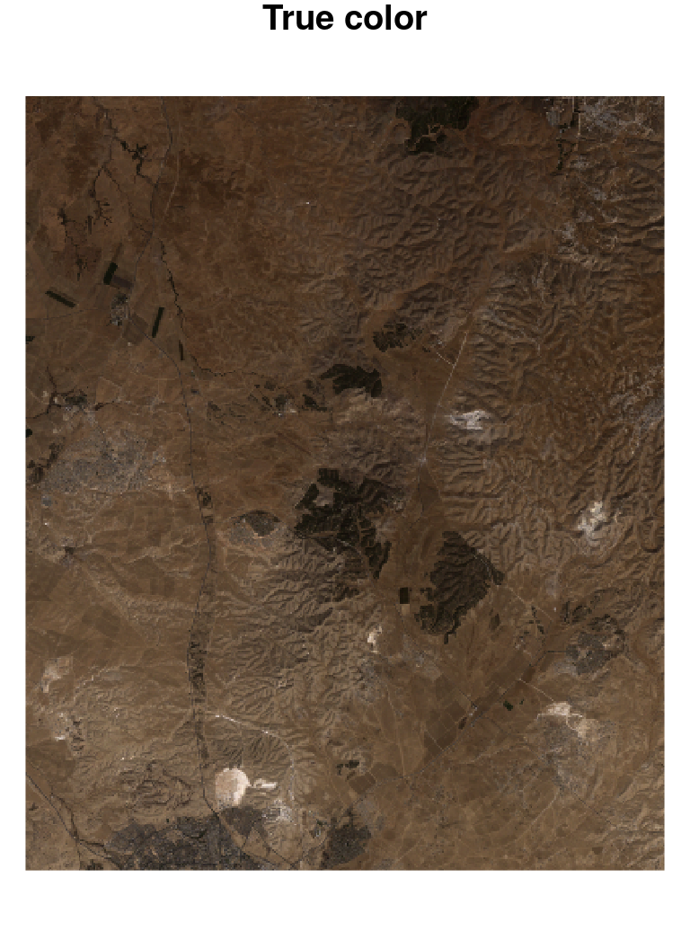

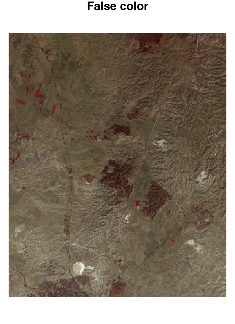
Figure 6.21: True color (left) and false color (right) images

6.4.4 Calculating NDVI

Multi-spectral images are commonly transformed to single band images using a spectral index. A common example of such an index is the NDVI, which we are familiar with from the raster MOD13A3_2000_2019.tif (Section 5.3.6). NDVI is defined as the difference between NIR and Red reflectance, divided by their sum (Equation (6.1)).

\[\begin{equation} NDVI=\frac{NIR-Red}{NIR + Red} \tag{6.1} \end{equation}\]

We can calculate an NDVI image based on the red and NIR bands in the Landsat image l, using raster algebra, as follows:

red = l[,,,3, drop = TRUE]
nir = l[,,,4, drop = TRUE]
ndvi = (nir - red) / (nir + red)
names(ndvi) = "NDVI"

The resulting NDVI image is shown in Figure 6.22:

plot(ndvi, breaks = "equal", col = hcl.colors(11, "Spectral"))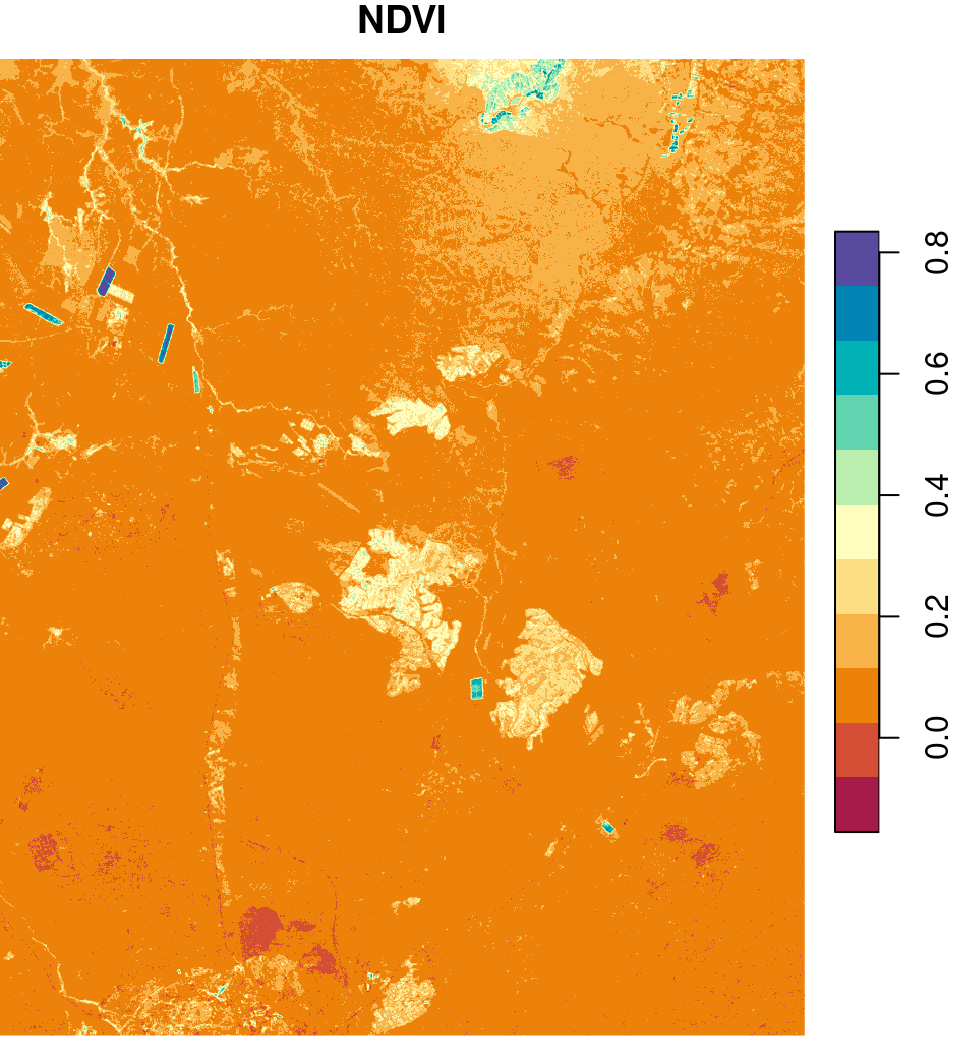

Figure 6.22: An NDVI image calculated based on a Landsat satellite image

6.5 Classification

Raster classification is the process of converting a continuous raster to a discrete one, by giving all pixels in a particular range of values a new uniform value (Figure 6.23).

Figure 6.23: Raster classification (http://rpubs.com/etiennebr/visualraster)

A raster can be classified, i.e., converted from a continuous raster to a categorical one, by assigning a new value to distinct ranges of the original values. For example, we can reclassify the continuous NDVI raster into two categories:

Low ($NDVI\leq0.2$) get the value of 0
High ($NDVI>0.2$) get the value of 1

Here is how we can do this with R code:

l_rec = ndvi
l_rec[ndvi <= 0.2] = 0
l_rec[ndvi > 0.2] = 1

The result is shown in Figure 6.24 ²⁵:

plot(l_rec, col = c("grey90", "darkgreen"))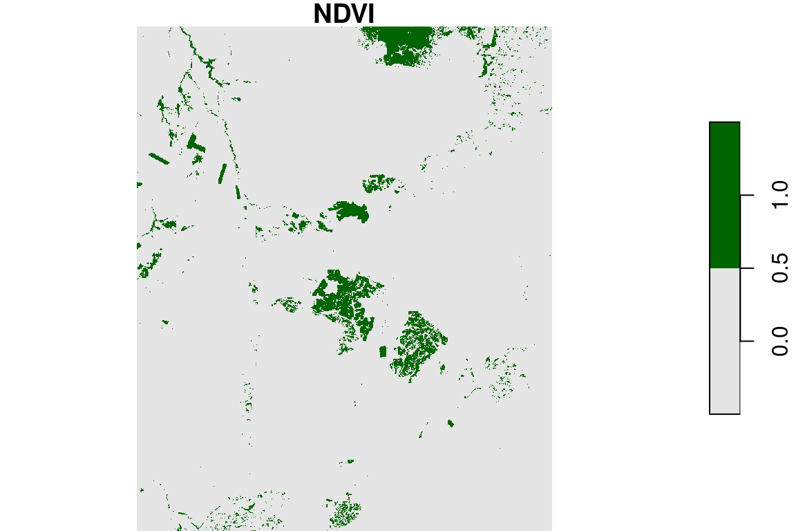

Figure 6.24: Reclassified NDVI image

6.6 Generalizing raster algebra with `st_apply`

6.6.1 Operating on each pixel

6.6.1.1 Introduction

Suppose that we have a small raster named s, with two layers:

s = r[, 99:101, 202:204, 1:2]
s[[1]]
## , , 1
## 
##        [,1]   [,2]   [,3]
## [1,] 0.2404 0.2313 0.2452
## [2,] 0.2513 0.2584 0.2564
## [3,] 0.2735     NA     NA
## 
## , , 2
## 
##        [,1]   [,2]   [,3]
## [1,] 0.2236 0.2375 0.2660
## [2,] 0.2680 0.2856 0.2563
## [3,] 0.2852 0.2746 0.2611

and that we would like to add up the two layers, plus a constant value of 10. We have already seen this is a raster algebra operation that can be achieved with arithmetic operators (Section 6.4.1):

u = s[,,,1,drop=TRUE] + s[,,,2,drop=TRUE] + 10
u[[1]]
##         [,1]    [,2]    [,3]
## [1,] 10.4640 10.4688 10.5112
## [2,] 10.5193 10.5440 10.5127
## [3,] 10.5587      NA      NA

But what if we want to apply a function on three, ten, or a hundred layers? Specifying each and every layer is impractical in such case. For that, we have a more general raster algebra approach using st_apply. The st_apply function is very similar to apply (Section 4.5). It takes an object, the dimension indices we wish to operate on, and a function, then applies the function on each subset along the dimension(s).

For example, the following expression calculates the same raster u as shown above, using st_apply:

u = st_apply(X = s, MARGIN = 1:2, FUN = function(x) sum(x) + 10)
u[[1]]
##         [,1]    [,2]    [,3]
## [1,] 10.4640 10.4688 10.5112
## [2,] 10.5193 10.5440 10.5127
## [3,] 10.5587      NA      NA

where function(x) sum(x)+10 is a function applied on the vector of values x of each pixel.

The FUN parameter determines the function which is going to be applied on each subset of the chosen dimension, just like in apply (Section 4.5). In case the dimension we operate on is 1:2, i.e., “pixels” (Section 5.2.3), the FUN parameter determines the function which calculates each pixel value in the output raster, given the respective pixel values of the input raster from all layers. The FUN function needs to accept a vector of any length and return a vector of length 1. As a result, st_apply returns a single-band raster with the calculated values for each pixel²⁶.

The st_apply function thus makes it possible to summarize raster dimension(s) properties using various built-in functions, such as mean, sum, min, max, etc., as well as custom functions (Section 3.3), such as function(x) sum(x)+10.

6.6.1.2 NDVI

As another example, the above expression to calculate NDVI (Section 6.4.4):

red = l[,,,3, drop = TRUE]
nir = l[,,,4, drop = TRUE]
ndvi = (nir - red) / (nir + red)

Can be replaced with the following analogous expression using st_apply:

ndvi = st_apply(l, 1:2, function(x) (x[4]-x[3])/(x[4]+x[3]))

6.6.1.3 Pixel means

Calculating pixel means, across all raster layers, is a very common operation with raster time series. The following expression uses st_apply along with FUN=mean to calculate a new raster with the average NDVI values (during the period 2000-2019) per pixel, based on the raster r. The additional na.rm=TRUE argument is passed to the function (mean, in this case). This makes the calculation ignore NA values:

s = st_apply(r, 1:2, mean, na.rm = TRUE)

The resulting average NDVI raster is shown in Figure 6.25:

plot(s, breaks = "equal", col = hcl.colors(11, "Spectral"))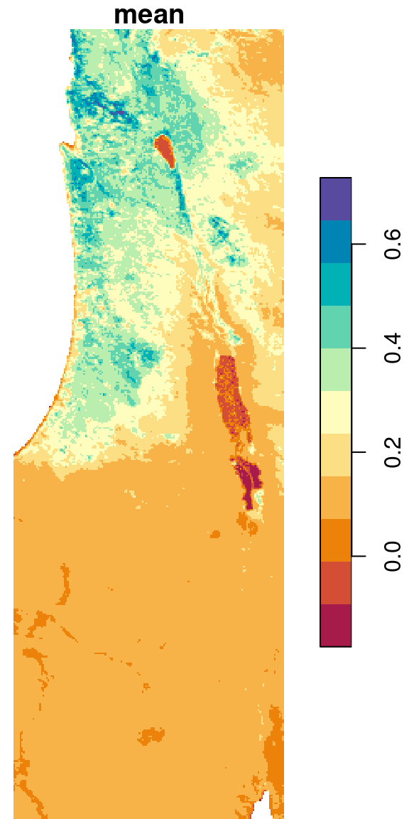

Figure 6.25: Average NDVI per pixel

6.6.1.4 Pixel minimum and maximum

In the following example, we use the min and max functions to calculate the minimal and maximal NDVI value, respectively, per pixel. In case our raster contains pixels where all values are NA, such as the case in r (6.6.1.6), we need to use slightly modified versions of min and max to avoid returning Inf and -Inf for those pixels:

min(c(NA, NA, NA), na.rm = TRUE)
## [1] Inf

max(c(NA, NA, NA), na.rm = TRUE)
## [1] -Inf

The modified functions can be constructed as follows. In case all values are NA, the functions return NA. In case there is at least one non-NA value, the minimum or maximum is calculated:

min2 = function(x) if(all(is.na(x))) NA else min(x, na.rm = TRUE)
max2 = function(x) if(all(is.na(x))) NA else max(x, na.rm = TRUE)

Let’s see if the new functions work as expected:

min2(c(NA, NA, NA, NA, NA))
## [1] NA
min2(c(NA, 24, NA, 20, NA))
## [1] 20

max2(c(NA, NA, NA, NA, NA))
## [1] NA
max2(c(NA, 24, NA, 20, NA))
## [1] 24

Now we can apply min2 and max2 on each pixel, to obtain single-band rasters with the minimum and maximum per pixel:

s_min = st_apply(r, 1:2, min2)
s_max = st_apply(r, 1:2, max2)

The results are shown in Figure 6.26:

plot(s_min, breaks = "equal", col = hcl.colors(11, "Spectral"), key.pos = 4)
plot(s_max, breaks = "equal", col = hcl.colors(11, "Spectral"), key.pos = 4)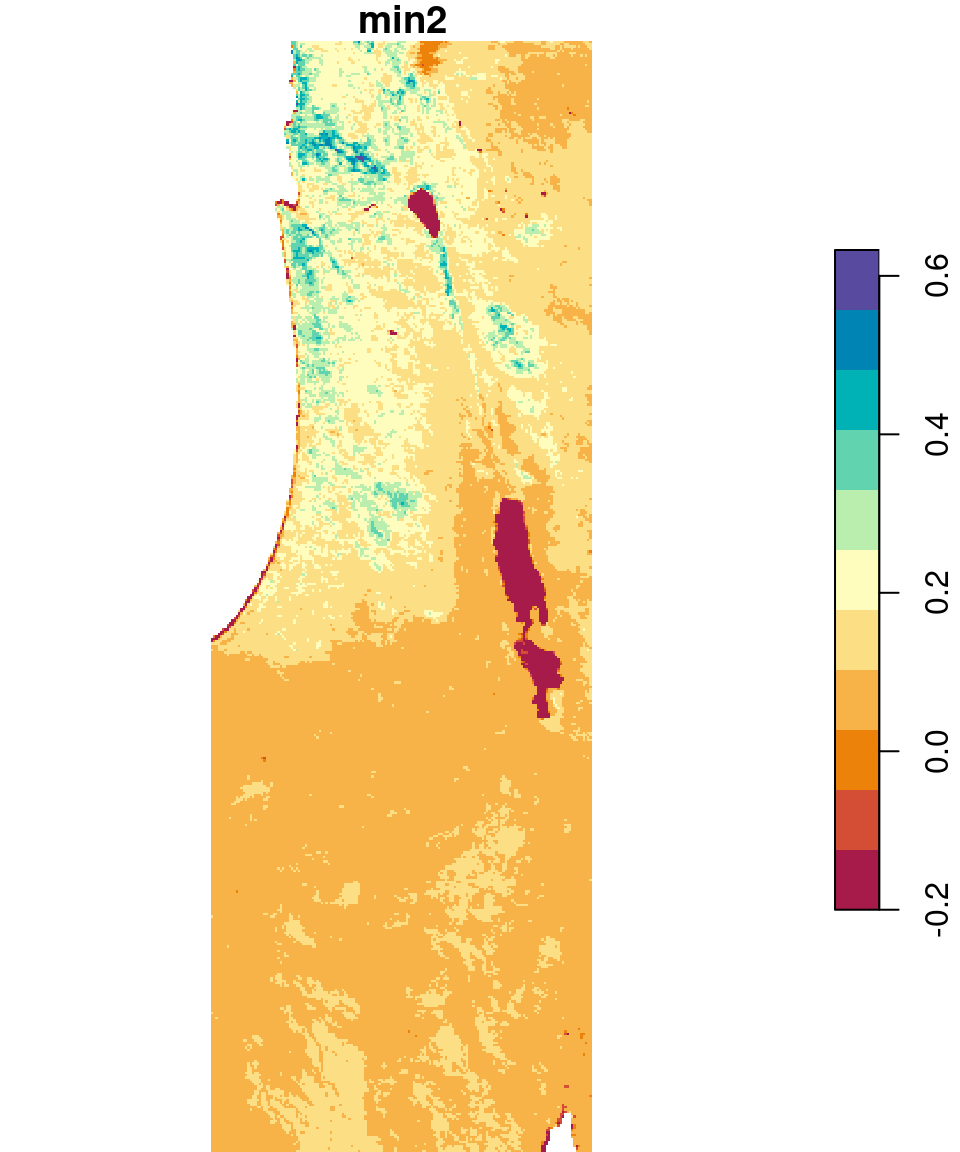

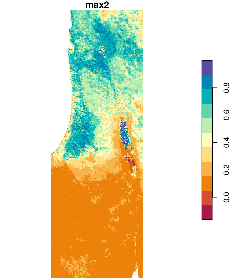
Figure 6.26: Minimum and maximum NDVI value per pixel

6.6.1.5 Pixel amplitudes

We can take the result from Section 6.6.1.4 and further calculate the difference between the maximum and minimum NDVI, i.e., the observed amplitude of NDVI values, in the raster r. This is yet another example of an arithmetic operator in raster algebra (Section 6.4.1):

s = s_max - s_min
names(s) = "amplitude"

The result is shown in Figure 6.27:

plot(s, breaks = "equal", col = hcl.colors(11, "Spectral"))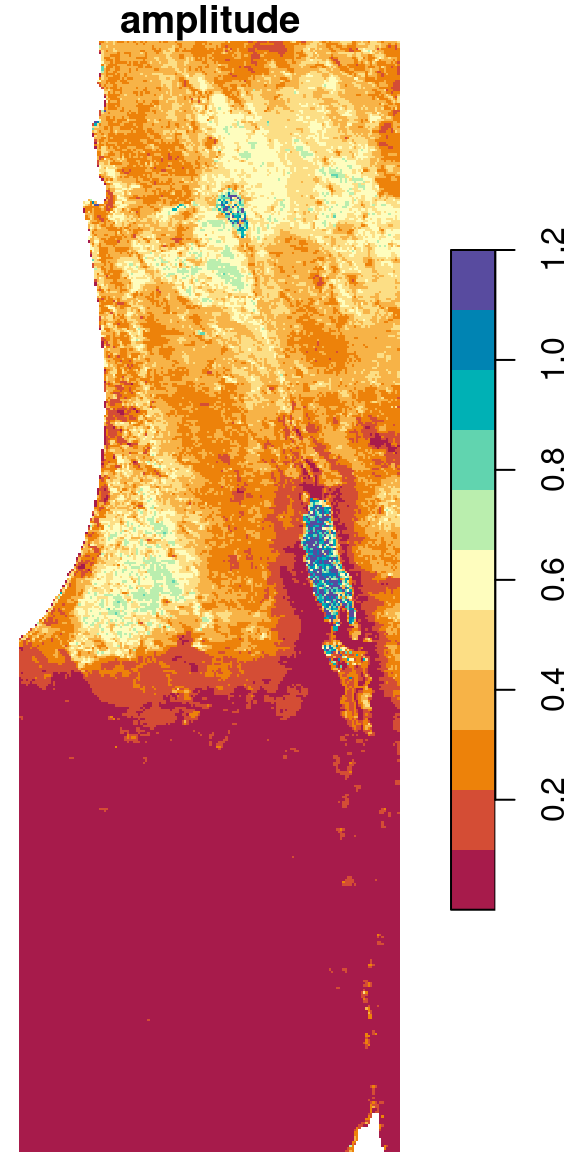

Figure 6.27: Amplitude of NDVI values per pixel

6.6.1.6 Pixel `NA` proportions

Another practical use case for st_apply is calculating the proportion of NA values per pixel:

s = st_apply(r, 1:2, function(x) mean(is.na(x)))
names(s) = "Proportion of NA values"

The result is a raster with values between 0 and 1, where 0 means none of the 233 values of that pixel are NA, and 1 means that all 233 values are NA. The raster is shown in Figure 6.28. The second expression uses contour (Section 5.1.6) to highlight the areas where more than 5% of the pixel values are NA:

plot(s, breaks = "equal", col = hcl.colors(100, "Spectral"), reset = FALSE)
contour(s, levels = 0.05, add = TRUE)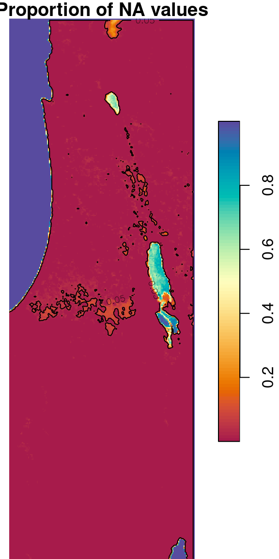

Figure 6.28: Proportion of NA values per pixel

6.6.2 Operating on each layer

In Section 6.6.1 we have seen examples of applying a function on the value of each pixel, using MARGIN=1:2. Another useful mode of operation with st_apply is summarizing the properties of each layer, rather than each pixel. This is achieved with MARGIN=3. For example, the following expressions calculate the minimum, mean and maximum NDVI value across the entire image per layer (i.e., per month):

layer_mean = st_apply(r, 3, mean, na.rm = TRUE)
layer_min = st_apply(r, 3, min, na.rm = TRUE)
layer_max = st_apply(r, 3, max, na.rm = TRUE)

The resulting stars objects are one-dimensional. Accordingly, layer_mean[[1]], layer_min[[1]] and layer_max[[1]] are one-dimensional arrays. One-dimensional arrays are treated as numeric vectors in most cases. For example, the following expression returns the average NDVI values of the first 10 layers in r:

layer_mean[[1]][1:10]
##  [1] 0.2023428 0.2263248 0.2298939 0.1923323 0.1580042 0.1510594 0.1482469
##  [8] 0.1443631 0.1496102 0.1650173

The three resulting time series can therefore be visualized as follows (Figure 6.29):

times = st_get_dimension_values(r, "time")
plot(times, layer_mean[[1]], type = "o", ylim = range(r[[1]], na.rm = TRUE), xlab = "Time", ylab = "NDVI")
lines(times, layer_min[[1]], type = "o", col = "blue")
lines(times, layer_max[[1]], type = "o", col = "red")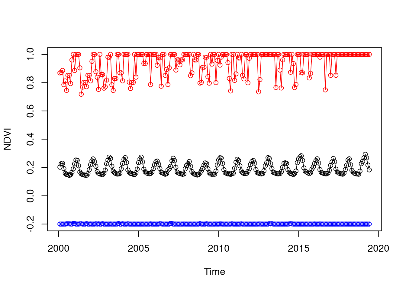

Figure 6.29: Minimum, mean and maximum NDVI over time

https://landsat.usgs.gov/what-are-band-designations-landsat-satellites ↩︎
This type of a false color image mapping emphasizes green vegetation (in red).↩︎
We can also do the above reclassification with a single expression, using cut(ndvi, breaks = c(-Inf, 0.2, Inf)). This becomes especially convenient if we have numerous categories or classes. The result consists of values of type factor, which we don’t go into in this book.↩︎
st_apply also accepts vector of (fixed) length n larger than 1, in which case st_apply returns a multi-band raster with n layers.↩︎