Chapter 12 Spatial interpolation of point data

Last updated: 2021-03-31 00:28:11

Aims

Our aims in this chapter are:

Calculate an empirical variogram
Fit a variogram model
Interpolate using three methods:
- Inverse Distance Weighted (IDW) interpolation
- Ordinary Kriging (OK)
- Universal Kriging (UK)
Evaluate interpolation accuracy using Leave-One-Out Cross Validation

We will use the following R packages:

sf
stars
gstat
automap

12.1 What is spatial interpolation?

12.1.1 Interpolation models

Spatial interpolation is the prediction of a given phenomenon in unmeasured locations (Figures 12.1–12.2). For that, we need a spatial interpolation model—a set of procedures to calculate predicted values of the variable of interest, given calibration data.

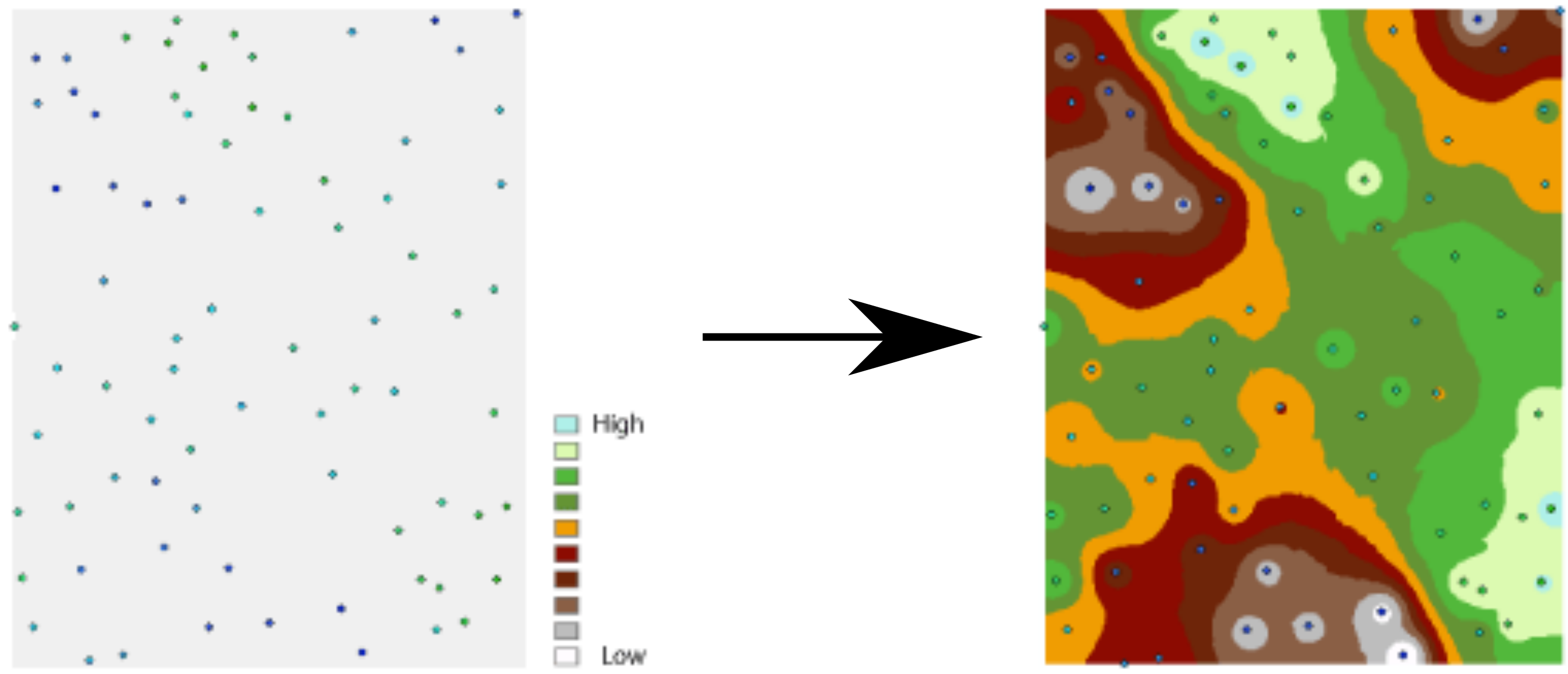
Spatial interpolation (Input elevation point data, Interpolated elevation surface) (http://desktop.arcgis.com/en/arcmap/10.3/tools/spatial-analyst-toolbox/understanding-interpolation-analysis.htm)

Figure 12.1: Spatial interpolation (Input elevation point data, Interpolated elevation surface) (http://desktop.arcgis.com/en/arcmap/10.3/tools/spatial-analyst-toolbox/understanding-interpolation-analysis.htm)

Spatial interpolation (Point locations of ozone monitoring stations, Interpolated prediction surface) (http://desktop.arcgis.com/en/arcmap/10.3/tools/spatial-analyst-toolbox/understanding-interpolation-analysis.htm)

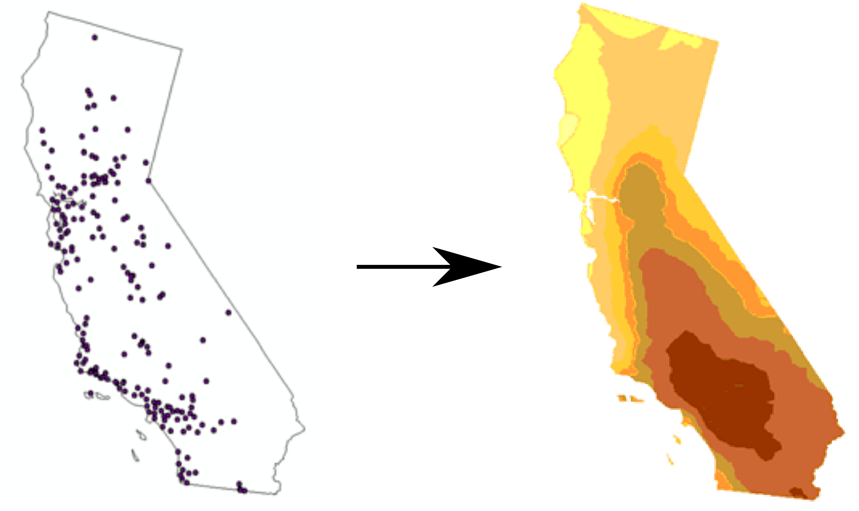
Figure 12.2: Spatial interpolation (Point locations of ozone monitoring stations, Interpolated prediction surface) (http://desktop.arcgis.com/en/arcmap/10.3/tools/spatial-analyst-toolbox/understanding-interpolation-analysis.htm)

Calibrarion data usually include:

Field measurements—available for a limited number of locations, for example: rainfall data from meteorological stations
Covariates—available for each and every location within the area of interest, for example: elevation from a DEM

Spatial interpolation models can be divided into two general categories:

Deterministic models—Models using arbitrary parameter values, for example: IDW
Statistical models—Models using parameters chosen objectively based on the data, for example: Kriging

Keep in mind that data structure does not imply meaning. It is technically possible to interpolate any numeric variable measured in a set of points, however it does not always make sense to do so. For example, it does not make sense to spatially interpolate point data when they refer to a localized phenomenon, such as amount of emissions per power plant (Figure 12.3).

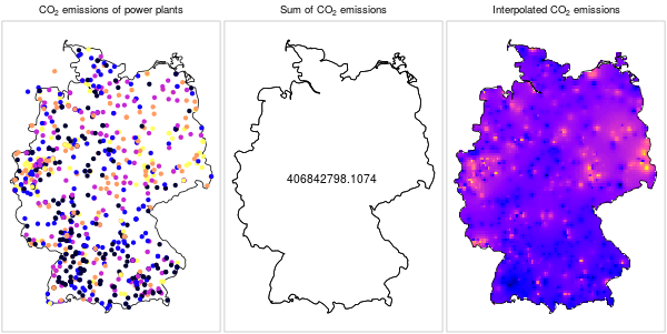
Figure 12.3: $CO_2$ emissions from power plants: a localized phenomenon (https://edzer.github.io/UseR2016/)

Converesly, it does not make sense to sum up point measurements of a continuous phenomenon (Figure 12.4).

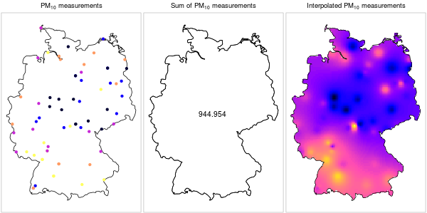
$$PM_{10}$ measurements: a continuous phenomenon (https://edzer.github.io/UseR2016/)$

Figure 12.4: $PM_{10}$ measurements: a continuous phenomenon (https://edzer.github.io/UseR2016/)

12.1.2 The weighted average principle

Many of the commonly used interpolation methods, including the ones we learn about in this Chapter (Nearest Neighbor, IDW, Kriging), are based on the same principle, where a predicted value is a weighted average of neighboring points. Weight are usually inveresely related to distance, i.e., as distance increases the weight (importance) of the point decreases. The predicted value for a particular point is calculated as a weighted average of measured values in other points (Equation (12.1)):

\[\begin{equation} \hat{Z}(s_{0})=\frac{\sum_{i=1}^{n}w(s_{i})Z(s_{i})}{\sum_{i=1}^{n}w(s_{i})} \tag{12.1} \end{equation}\]

where:

$\hat{Z}(s_{0})$ is the predicted value at location $s_{0}$
$w(s_{i})$ is the weight of measured point $i$
$Z(s_{i})$ is the value of measured point $i$

The weight $w(s_{i})$ of each measured point is a function of distance (Figure 12.5) from the predicted point.

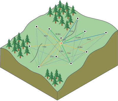
Distances between predicted point and all measured points (http://desktop.arcgis.com/en/arcmap/10.3/tools/spatial-analyst-toolbox/how-kriging-works.htm)

Figure 12.5: Distances between predicted point and all measured points (http://desktop.arcgis.com/en/arcmap/10.3/tools/spatial-analyst-toolbox/how-kriging-works.htm)

In IDW, the weight is the inverse of distance to the power of $p$ (Equation (12.2)):

\[\begin{equation} w(s_{i})=\frac{1}{d(s_{0}, s_{i})^p} \tag{12.2} \end{equation}\]

where:

$w(s_{i})$ is the weight of measured point $i$
$d(s_{0}, s_{i})$ is the distance between predicted point $s_{0}$ and measured point $s_{i}$

The default value for $p$ is usually $p=2$ (Equation (12.3)):

\[\begin{equation} w(s_{i})=\frac{1}{d(s_{0}, s_{i})^2} \tag{12.3} \end{equation}\]

The $p$ parameter basically determines how steeply does weight increase with proximity. As a result, $p$ determines whether weights are more or less equally distributed among neighbors (low $p$) or whether one point (the nearest) has overwhelmingly high weight and thus the predicted value will be strongly influenced by that point (high $p$). In other words, when $p$ approaches zero, the predicted result will approach a uniform surface which is just an average of all measured points. When $p$ approaches infinity, the predicted result will approach nearest neighbor interpolation, which is the simplest spatial interpolation method there is: every predicted point gets the value of the nearest measured point (Figures 12.6–12.7).

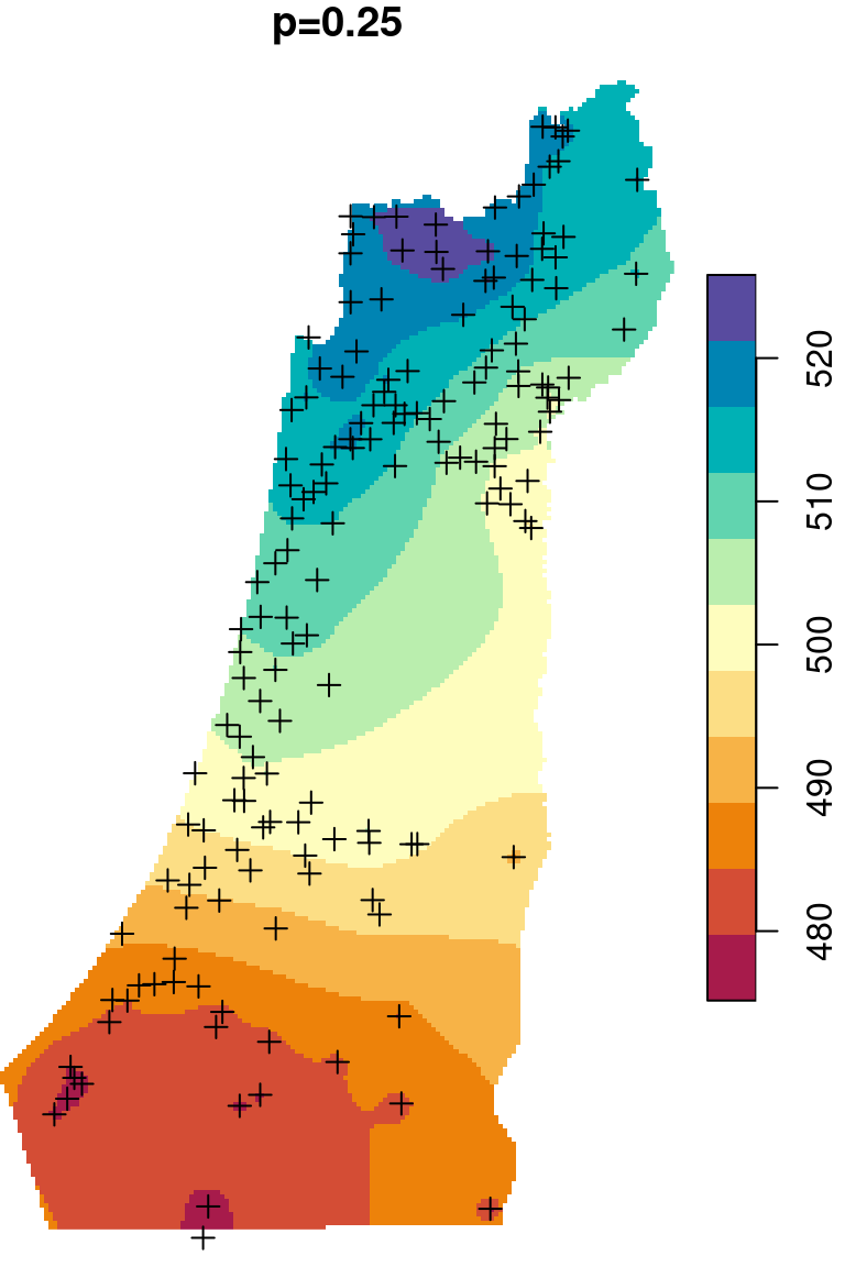
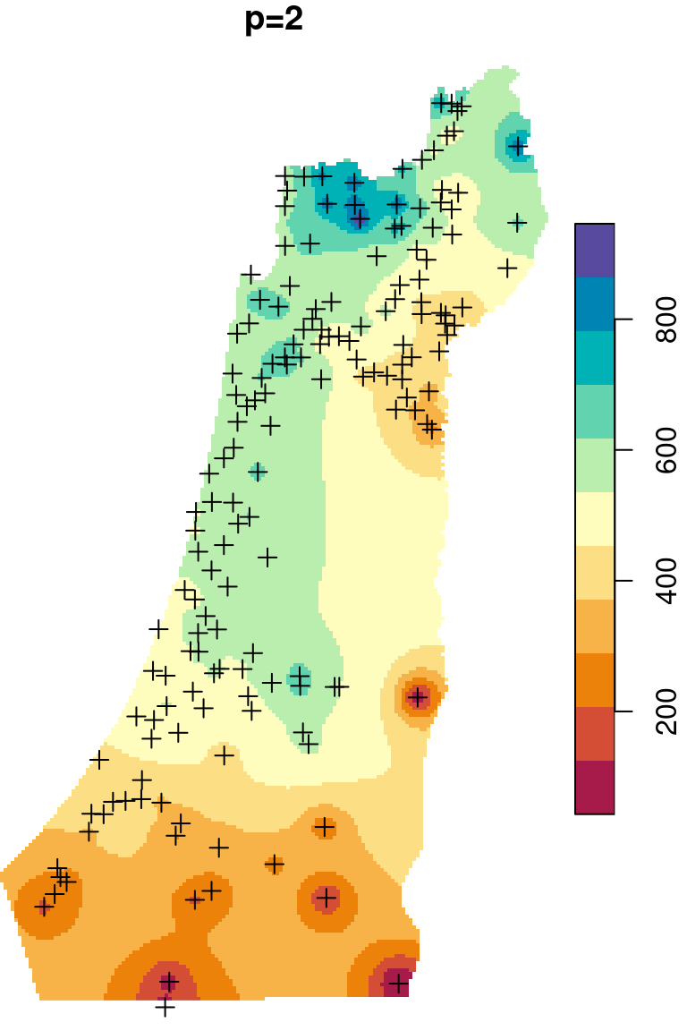
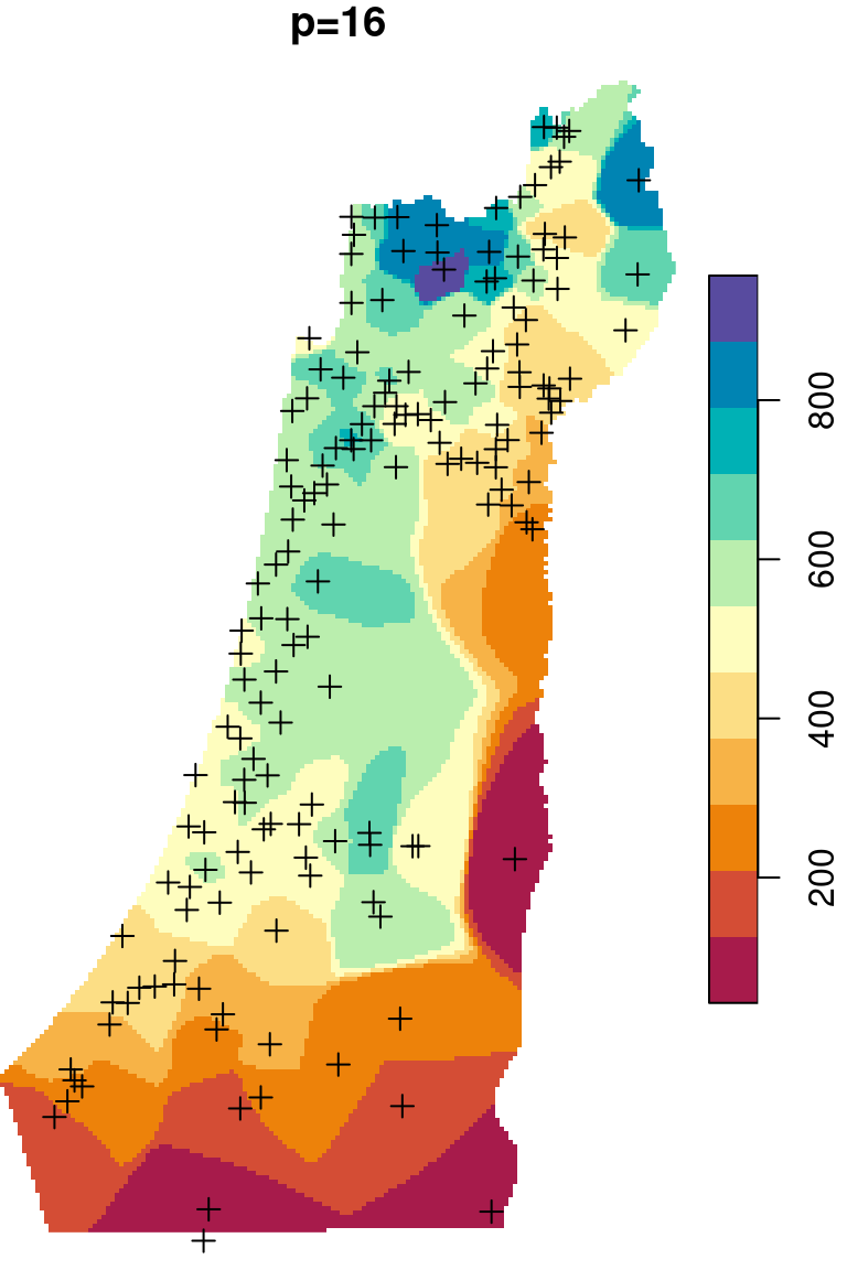
Spatial interpolation of annual rainfall using IDW with $p=0.25$, $p=2$ and $p=16$

Figure 12.6: Spatial interpolation of annual rainfall using IDW with $p=0.25$, $p=2$ and $p=16$

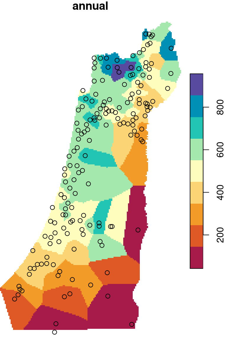
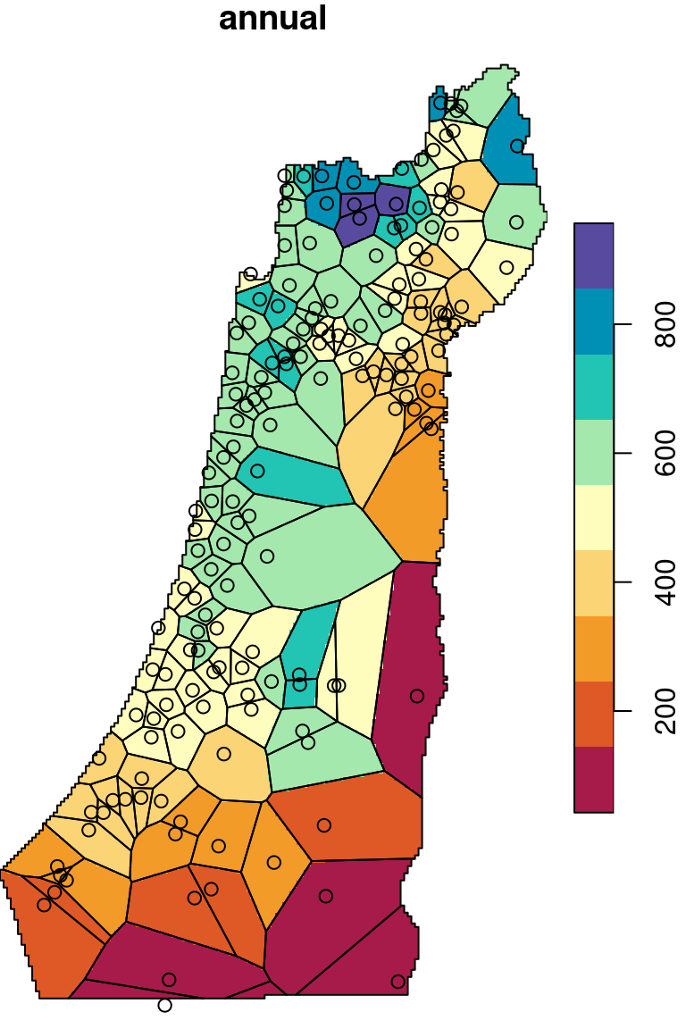
Figure 12.7: Nearest Neighbor interpolation (left) and Voronoi polygons (right)

In Kriging, the weight is a particular function of distance known as the variogram model (Figure 12.8). The variogram model is fitted to characterize the autocorrelation structure in the measured data, based on the empirical variogram.

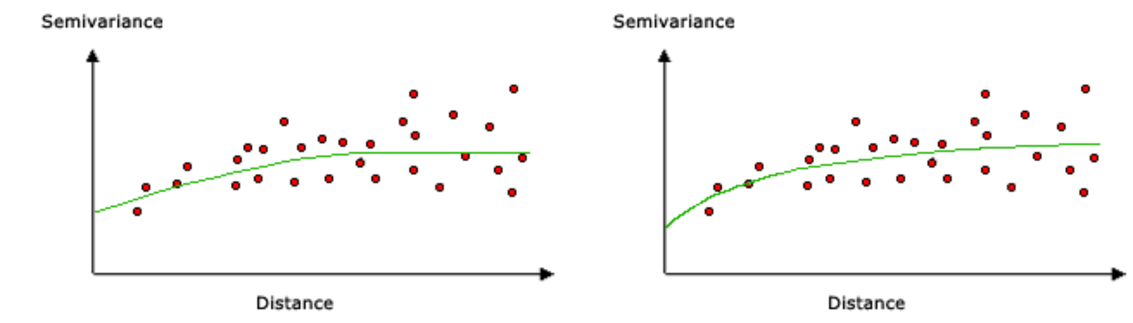
Variogram models: spherical (left) and exponential (right) (http://desktop.arcgis.com/en/arcmap/10.3/tools/spatial-analyst-toolbox/how-kriging-works.htm)

Figure 12.8: Variogram models: spherical (left) and exponential (right) (http://desktop.arcgis.com/en/arcmap/10.3/tools/spatial-analyst-toolbox/how-kriging-works.htm)

There are two frequently used kriging methods: Ordinary Kriging (OK) and Universal Kriging (UK). Adding up the Inverse Distance Weighted (IDW) interpolation, we now mentioned three interpolation methods. We are going to cover those three methods (Figure 12.9), mostly from the practical point of view, in the next three sections (Sections 12.2–12.4).

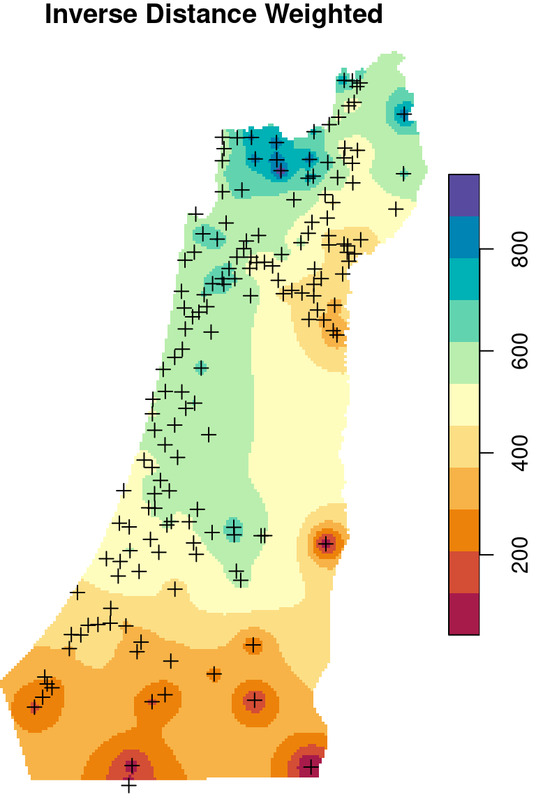
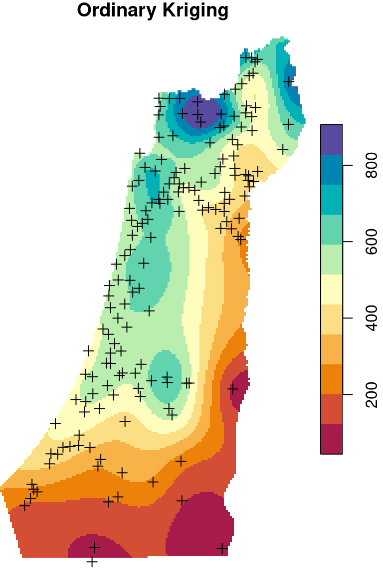
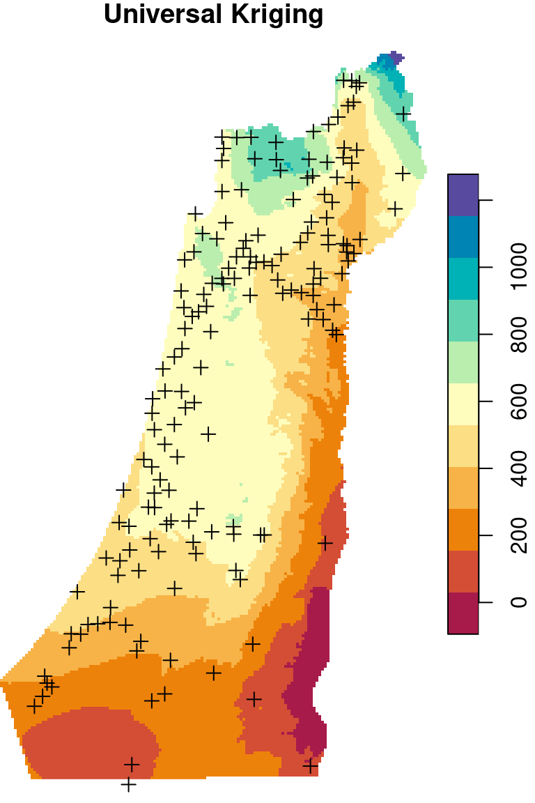
Spatial interpolation of annual rainfall using IDW, OK and UK

Figure 12.9: Spatial interpolation of annual rainfall using IDW, OK and UK

For the examples, we will load the rainfall.csv file (Section 4.4.3), calculate the annual column (Section 4.5) and convert it to a point layer (Section 7.4):

library(sf)
rainfall = read.csv("rainfall.csv")
rainfall = st_as_sf(rainfall, coords = c("x_utm", "y_utm"), crs = 32636)
m = c("sep", "oct", "nov", "dec", "jan", "feb", "mar", "apr", "may")
rainfall$annual = apply(st_drop_geometry(rainfall[, m]), 1, sum)

We will also use a $1\times1$ $km^2$ DEM raster of the area of interest (Sections 9.1, 9.3 and 10.1):

library(stars)
dem1 = read_stars("srtm_43_06.tif")
dem2 = read_stars("srtm_44_06.tif")
dem = st_mosaic(dem1, dem2)
borders = st_read("israel_borders.shp")
grid = st_as_sfc(st_bbox(borders))
grid = st_as_stars(grid, dx = 1000, dy = 1000)
dem = st_warp(src = dem, grid, method = "average", use_gdal = TRUE)
dem = dem[borders]
names(dem) = "elev_1km"

Finally, we subset the dem to include only the area to the north of 31 degrees latitude, where meteorological station density is relatively high:

y = st_as_sf(dem, as_points = TRUE)
y$lat = st_coordinates(st_transform(y, 4326))[,2]
y = st_rasterize(y[, "lat"], dem)
y[y < 31] = NA
y[!is.na(y)] = 1
y = st_as_sf(y, merge = TRUE)
dem = dem[y]

Next, we extract the elevation values (Section 10.7.2):

rainfall = st_join(rainfall, st_as_sf(dem))

and subset those stations that coincide with the raster:

rainfall = rainfall[!is.na(rainfall$elev_1km), ]

Figure 12.10 shows the dem elevation raster and the rainfall point layer:

plot(dem, breaks = "equal", col = terrain.colors(11), reset = FALSE)
plot(st_geometry(rainfall), add = TRUE)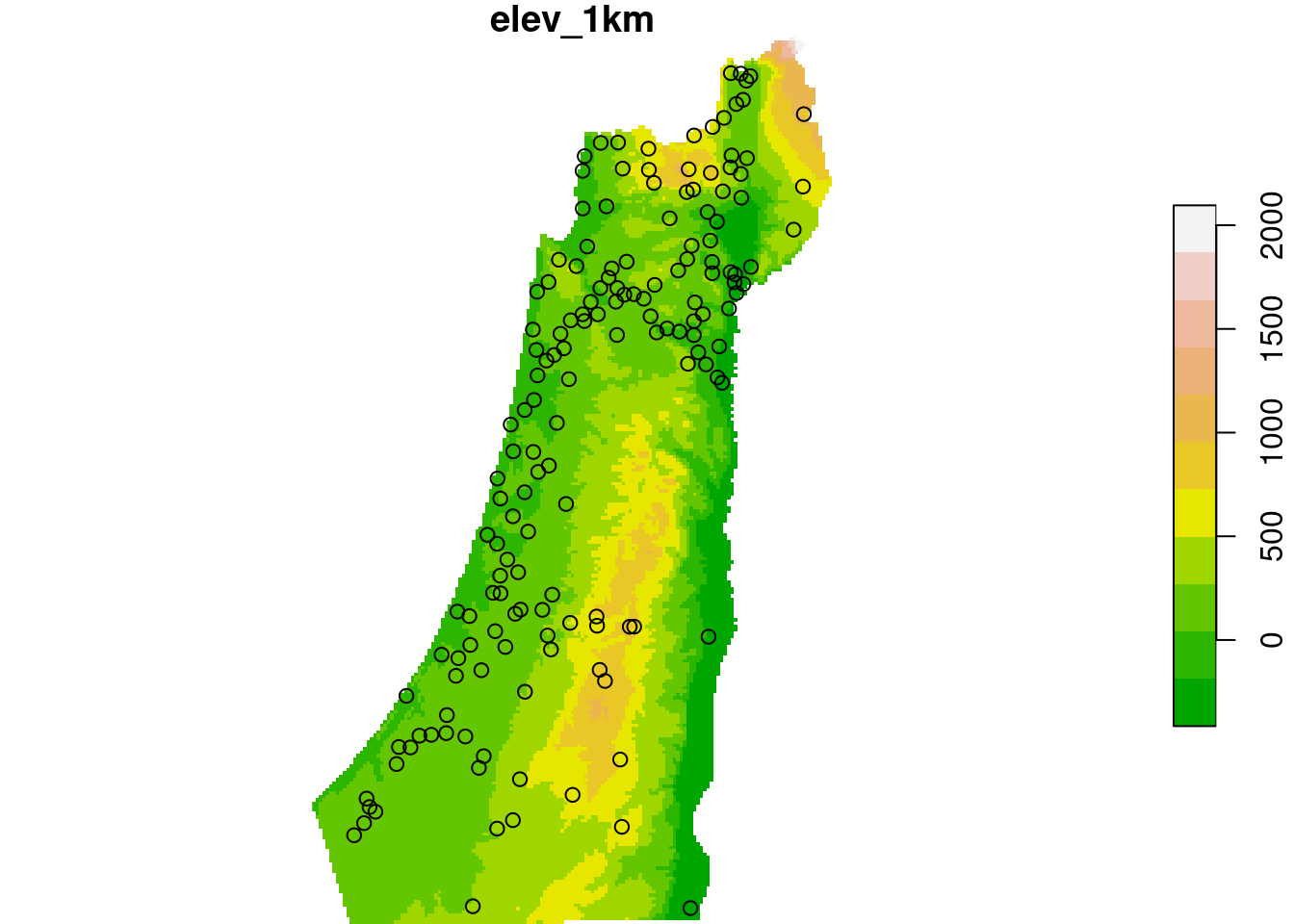

Figure 12.10: Rainfall data points and elevation raster

12.2 Inverse Distance Weighted interpolation

12.2.1 The `gstat` object

To interpolate, we first need to create an object of class gstat, using a function of the same name: gstat. A gstat object contains all necessary information to conduct spatial interpolation, namely:

The model definition
The calibration data

Based on its arguments, the gstat function “understands” what type of interpolation model we want to use:

No variogram model → IDW
Variogram model, no covariates → Ordinary Kriging
Variogram model, with covariates → Universal Kriging

The complete decision tree of gstat, including several additional methods which we are not going to use, is shown in Figure 12.11.

Figure 12.11: gstat predict methods (Applied Spatial Data Analysis with R, 2013)

We are going to use three parameters of the gstat function:

formula—The prediction “formula” specifying the dependent and the independent variables (covariates)
data—The calibration data
model—The variogram model

Keep in mind that we need to specify parameter names, because these three parameters are not the first three in the gstat function definition.

For example, to interpolate using the IDW method we create the following gstat object, specifying just the formula (Section 12.2.2 below) and data:

library(gstat)
g = gstat(formula = annual ~ 1, data = rainfall)

12.2.2 Working with `formula` objects

Im R, formula objects are used to specify relation between objects, in particular—the role of different data columns in statistical models. A formula object is created using the ~ operator, which separates names of dependent variables (to the left of the ~ symbol) and independent variables (to the right of the ~ symbol). Writing 1 to the right of the ~ symbol, as in ~ 1, means that there are no independent variables³⁹.

For example, in the following expression we create a formula object named f:

f = annual ~ 1
f
## annual ~ 1

Checking the class shows that f is indeed a formula object:

class(f)
## [1] "formula"

We can also convert character values to formula using the as.formula function. For example:

f = as.formula("annual ~ 1")
class(f)
## [1] "formula"

The as.formula function is particularly useful when we want to construct different formulas as part of a for loop (Section 12.3.3).

12.2.3 Making predictions

Now that our model is defined, we can use the predict function to actually interpolate, i.e., to calculate predicted values. The predict function accepts:

A raster—stars object, such as dem
A model—gstat object, such as g

The raster serves for two purposes:

Specifying the locations where we want to make predictions (in all methods)
Specifying covariate values (in Universal Kriging only)

For example, the following expression interpolates annual values according to the model defined in g and the raster template defined in dem:

z = predict(g, dem)
## [inverse distance weighted interpolation]

The resulting stars object has two attributes:

var1.pred—the predicted values
var1.var—the variance (for Kriging only)

For example:

z
## stars object with 2 dimensions and 2 attributes
## attribute(s):
##    var1.pred        var1.var     
##  Min.   : 42.85   Min.   : NA    
##  1st Qu.:356.01   1st Qu.: NA    
##  Median :495.20   Median : NA    
##  Mean   :466.49   Mean   :NaN    
##  3rd Qu.:552.16   3rd Qu.: NA    
##  Max.   :946.31   Max.   : NA    
##  NA's   :20108    NA's   :39933  
## dimension(s):
##   from  to  offset delta                       refsys point values x/y
## x    1 153  616965  1000 +proj=utm +zone=36 +datum...    NA   NULL [x]
## y    1 261 3691819 -1000 +proj=utm +zone=36 +datum...    NA   NULL [y]

We can subset just the first attribute and rename it to "annual":

z = z["var1.pred",,]
names(z) = "annual"

The interpolated annual rainfall raster, using IDW, is shown in Figure 12.12:

b = seq(0, 1200, 100)
plot(z, breaks = b, col = hcl.colors(length(b)-1, "Spectral"), reset = FALSE)
plot(st_geometry(rainfall), pch = 3, add = TRUE)
contour(z, breaks = b, add = TRUE)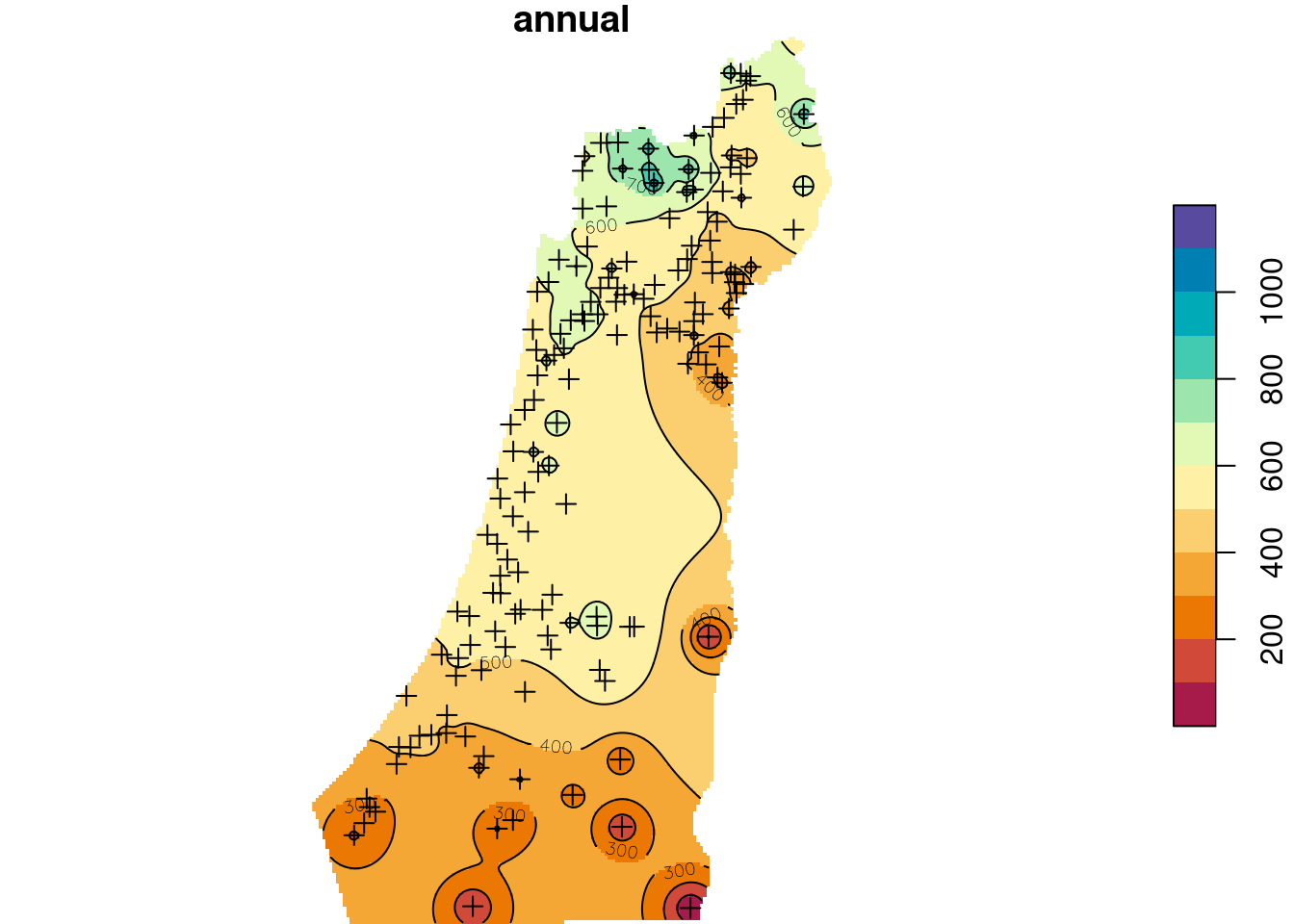

Figure 12.12: Predicted annual rainfall using Inverse Distance Weighted (IDW) interpolation

12.3 Ordinary Kriging

12.3.1 Annual rainfall example

Kriging methods require a variogram model. The variogram model is an objective way to quantify the autocorrelation pattern in the data, and assign weights accordingly when making predictions (Section 12.1.2).

As a first step, we can calculate and examine the empirical variogram using the variogram function. The function requires two arguments:

formula—Specifies the dependent variable and the covariates, just like in gstat
data—The point layer with the dependent variable and covariates as point attributes

For example, the following expression calculates the empirical variogram of annual, with no covariates:

v_emp_ok = variogram(annual ~ 1, rainfall)

Using plot to examine it we can examine the variogram (Figure 12.13):

plot(v_emp_ok)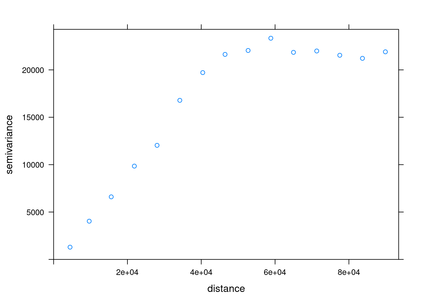

Figure 12.13: Empirical variogram

There are several ways to fit a variogram model to an empirical variogram. We will use the simplest one—automatic fitting using function autofitVariogram from package automap:

library(automap)
v_mod_ok = autofitVariogram(annual ~ 1, as(rainfall, "Spatial"))

The function chooses the best fitting type of model, and also fine tunes its parameters. (Use show.vgms() to display variogram model types.) Note that the autofitVariogram function does not work on sf objects, which is why we convert the object to a SpatialPointsDataFrame (package sp).

The fitted model can be plotted with plot (Figure 12.14):

plot(v_mod_ok)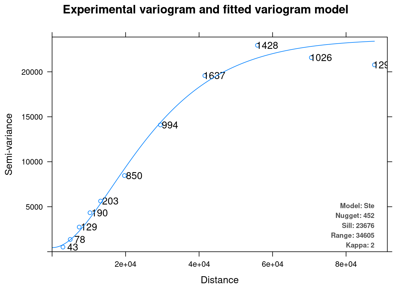

Figure 12.14: Variogram model

The resulting object is actually a list with several components, including the empirical variogram and the fitted variogram model. The $var_model component of the resulting object contains the actual model:

v_mod_ok$var_model
##   model      psill    range kappa
## 1   Nug   451.9177     0.00     0
## 2   Ste 23223.8370 34604.87     2

The variogram model can then be passed to the gstat function, and we can carry on with the Ordinary Kriging interpolation:

g = gstat(formula = annual ~ 1, model = v_mod_ok$var_model, data = rainfall)
z = predict(g, dem)
## [using ordinary kriging]

Again, we will subset the predicted values attribute and rename it:

z = z["var1.pred",,]
names(z) = "annual"

The Ordinary Kriging predictions are shown in Figure 12.15:

b = seq(0, 1200, 100)
plot(z, breaks = b, col = hcl.colors(length(b)-1, "Spectral"), reset = FALSE)
plot(st_geometry(rainfall), pch = 3, add = TRUE)
contour(z, breaks = b, add = TRUE)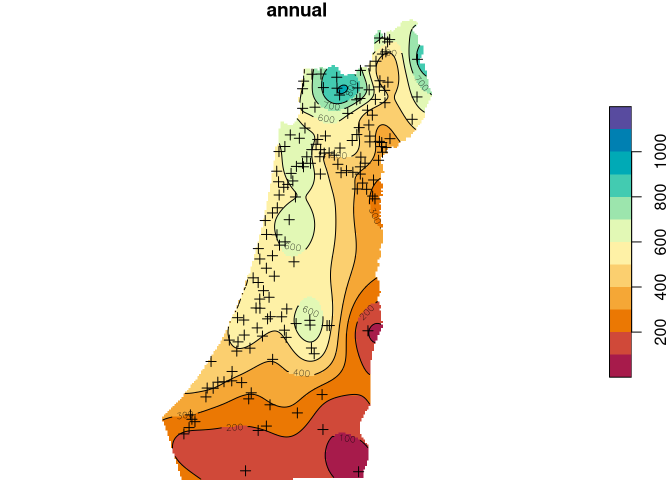

Figure 12.15: Predicted annual rainfall using Ordinary Kriging

12.3.2 Elevation example

Another example: suppose that we did not have a DEM for Israel, but only the elevation measurements at the meteorological stations. How can we produce an elevation raster using Ordinary Kriging?

First, we prepare the gstat object:

v = autofitVariogram(altitude ~ 1, as(rainfall, "Spatial"))
g = gstat(formula = altitude ~ 1, model = v$var_model, data = rainfall)

Then, we interpolate:

z = predict(g, dem)
## [using ordinary kriging]
z = z["var1.pred",,]
names(z) = "elevation"

The predicted elevation raster is shown in Figure 12.16:

b = seq(-500, 1200, 100)
plot(z, breaks = b, col = hcl.colors(length(b)-1, "Spectral"), reset = FALSE)
plot(st_geometry(rainfall), pch = 3, add = TRUE)
contour(z, breaks = b, add = TRUE)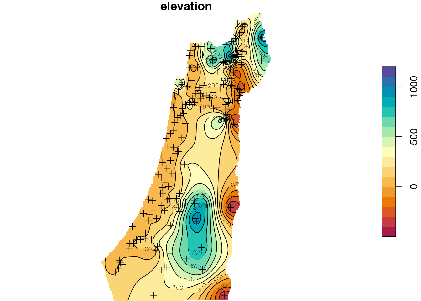

Figure 12.16: Ordinary Kriging prediction of elevation

12.3.3 Monthly rainfall example

In the next example we use kriging inside a for loop, to make a series of predictions for different variables. Specifically, we will use Ordinary Kriging to predict monthly rainfall, i.e., sep through may columns in the rainfall layer.

In each for loop “round,” the formula is going to be re-defined according to the current month i. For example:

i = "may"
as.formula(paste0(i, " ~ 1"))
## may ~ 1

First, we set up a vector with the column names of the variables we wish to interpolate, and a list where we “collect” the results:

m = c("sep", "oct", "nov", "dec", "jan", "feb", "mar", "apr", "may")
result = list()

Second, we specify the for loop, as follows:

for(i in m) {
  f = as.formula(paste0(i, " ~ 1"))
  v = autofitVariogram(f, as(rainfall, "Spatial"))
  g = gstat(formula = f, model = v$var_model, data = rainfall)
  z = predict(g, dem)
  z = z["var1.pred",,]
  result[[i]] = z
}
## [using ordinary kriging]
## [using ordinary kriging]
## [using ordinary kriging]
## [using ordinary kriging]
## [using ordinary kriging]
## [using ordinary kriging]
## [using ordinary kriging]
## [using ordinary kriging]
## [using ordinary kriging]

Finally, we combine the list of results per month into a single multi-band raster, using do.call and c (Section 11.3.2):

result$along = 3
result = do.call(c, result)

The interpolated montly rainfall amounts are shown in Figure 12.17:

plot(result, breaks = "equal", col = hcl.colors(11, "Spectral"), key.pos = 4)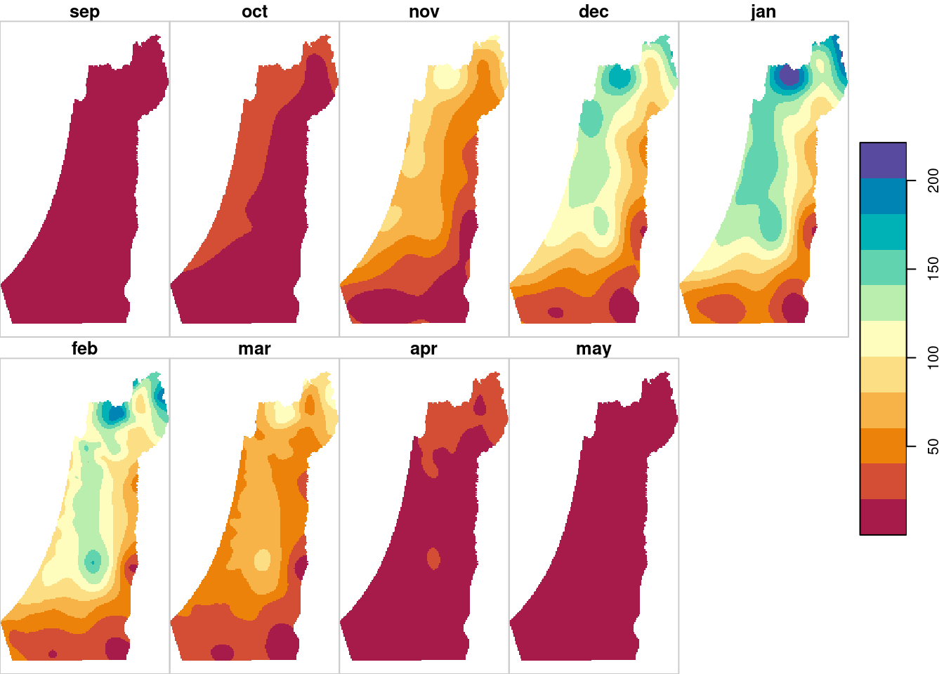

Figure 12.17: Monthly rainfall predictions using Ordinary Kriging

12.4 Universal Kriging

Universal Kriging interpolation uses a model with one or more independent variables, i.e., covariates. The covariates need to be known for both:

The point layer, as an attribute such as elev_1km in rainfall
The predicted locations, as raster values such as dem values

The formula now specifies the name(s) of the covariate(s) to the right of the ~ symbol, separated by + if there are more than one. Also, we are using a subset of rainfall where elev_1km values were present:

v_emp_uk = variogram(annual ~ elev_1km, rainfall)
v_mod_uk = autofitVariogram(annual ~ elev_1km, as(rainfall, "Spatial"))

Comparing the Ordinary Kriging and Universal Kriging variogram models (Figure 12.18):

plot(v_emp_ok, model = v_mod_ok$var_model, ylim = c(0, 25000), main = "OK")
plot(v_emp_uk, model = v_mod_uk$var_model, ylim = c(0, 25000), main = "UK")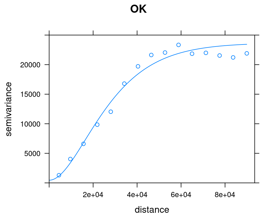

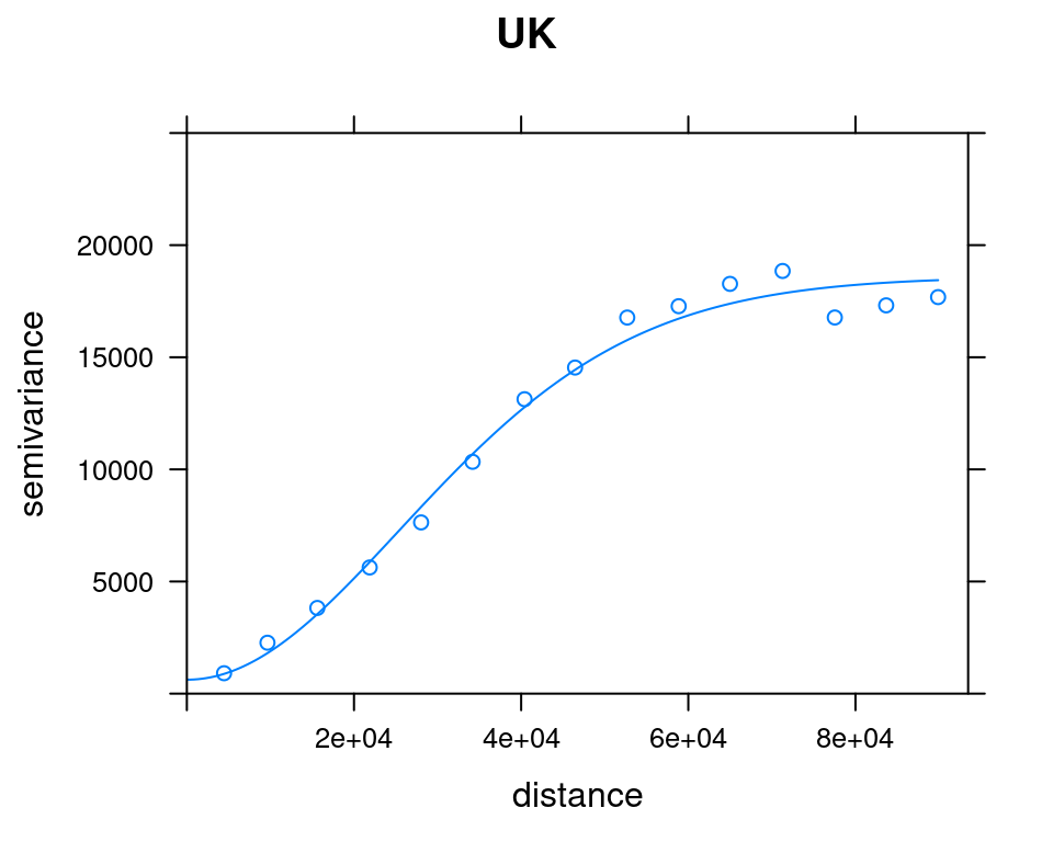
Figure 12.18: OK and UK variogram models

Next we create a gstat object, where the formula contains the covariate and the corresponding variogram model:

g = gstat(formula = annual ~ elev_1km, model = v_mod_uk$var_model, data = rainfall)

Remember that all of the variables that appear in the formula need to be present in the data. In this case we have two variables: a dependent variable (annual) and an independent variable (elev_1km).

Now we can make predictions:

z = predict(g, dem)
## [using universal kriging]

and then subset and rename:

z = z["var1.pred",,]
names(z) = "annual"

Universal Kriging predictions are shown in Figure 12.19:

b = seq(0, 1200, 100)
plot(z, breaks = b, col = hcl.colors(length(b)-1, "Spectral"), reset = FALSE)
plot(st_geometry(rainfall), pch = 3, add = TRUE)
contour(z, breaks = b, add = TRUE)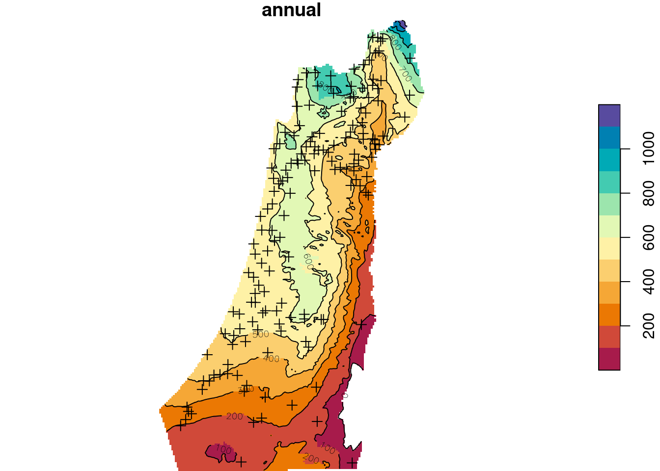

Figure 12.19: Predicted annual rainfall using Universal Kriging

12.5 Cross-validation

In Sections 12.2–12.4, we have calculated annual rainfall surfaces using three different methods: IDW, Ordinary Kriging and Universal Kriging. Although it is useful to examine and compare the results graphically (Figures 12.12, 12.15, and 12.19), we also need an objective way to evaluate interolation accuracy. That way, we can objectively choose the most accurate method among the various interpolation methods there are.

Plainly speaking, to evaluate prediction accuracy we need to compare the predicted values with measured data in the same location. Since measured data are often sparse and expensive to produce, it makes little sense to collect more data merely for the sake of accuracy assessment. Instead, the available data are usually split to two parst, called training and test data. The training data are used to fit the model, while the test data are used to calculate prediction accuracy. The procedure is called cross validation. A specific, commonly used, type of cross validation is Leave-One-Out Cross Validation where all observations consecutively take the role of test data while the remaning observations take the role of training data. The separation of training and test data is important because evaluating a model based on the same data used to fit it gives the model an “unfair” advantage and therefore overestimates accuracy.

In Leave-One-Out Cross Validation we:

Take out one point out of the calibration data
Make a prediction for that point
Repeat for all points

In the end, what we get is a table with an observed value and a predicted value for all points.

We can run Leave-One-Out Cross Validation using the gstat.cv function, which accepts a gstat object:

cv = gstat.cv(g)

The gstat.cv function returns an object of class SpatialPointsDataFrame (package sp), which we can convert to an sf object with st_as_sf:

cv = st_as_sf(cv)
cv
## Simple feature collection with 160 features and 6 fields
## Geometry type: POINT
## Dimension:     XY
## Bounding box:  xmin: 629301.4 ymin: 3435503 xmax: 761589.2 ymax: 3681163
## CRS:           NA
## First 10 features:
##    var1.pred var1.var observed    residual       zscore fold
## 1   632.4635 951.6388    582.8 -49.6635206 -1.609909413    1
## 2   614.6876 915.2690    608.5  -6.1876076 -0.204525930    2
## 3   598.0584 907.7003    614.7  16.6415723  0.552361147    3
## 4   609.5275 774.8052    562.7 -46.8274602 -1.682303431    4
## 5   701.0174 913.6664    682.8 -18.2174496 -0.602689676    5
## 6   610.4985 740.2553    705.5  95.0014929  3.491722024    6
## 7   645.4771 824.3927    610.4 -35.0771011 -1.221677615    7
## 8   581.9809 976.5117    583.3   1.3190893  0.042211954    8
## 9   654.7017 705.9952    709.8  55.0983188  2.073659677    9
## 10  654.6546 706.8918    654.8   0.1454226  0.005469598   10
##                    geometry
## 1  POINT (697119.1 3656748)
## 2  POINT (696509.3 3652434)
## 3  POINT (696541.7 3641332)
## 4  POINT (697875.3 3630156)
## 5  POINT (689553.7 3626282)
## 6  POINT (694694.5 3624388)
## 7  POINT (686489.5 3619716)
## 8  POINT (683148.4 3616846)
## 9  POINT (696489.3 3610221)
## 10 POINT (693025.1 3608449)

The result of gstat.cv has the following attributes:

var1.pred—Predicted value
var1.var—Variance (only for Kriging)
observed—Observed value
residual—Observed-Predicted
zscore—Z-score (only for Kriging)
fold—Cross-validation ID

A bubble plot is convenient to examine the residuals, since it shows positive and negative values in different color (Figure 12.20):

bubble(as(cv[, "residual"], "Spatial"))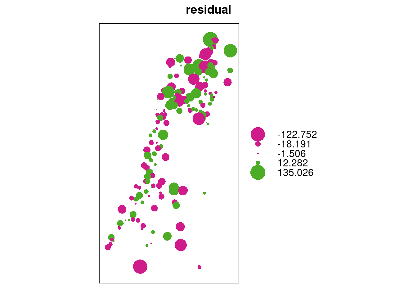

Figure 12.20: Cross-validation residuals

Using the “predicted” and “observed” columns we can calculate prediction accuracy indices, such as the Root Mean Square Error (RMSE) (Equation (12.4)):

\[\begin{equation} RMSE=\sqrt{\frac{\sum_{i=1}^{n} (pred_i-obs_i)^2}{n}} \tag{12.4} \end{equation}\]

where $pred_i$ and $obs_i$ are predicted and observed values for point $i$, respectively.