Chapter 7 Vector layers
Last updated: 2021-03-31 00:24:22
Aims
Our aims in this chapter are:
- Become familiar with data structures for vector layers: points, lines and polygons
- Examine spatial and non-spatial properties of vector layers
- Create subsets of vector layers based on their attributes
- Learn to transform a layer from one Coordinate Reference System (CRS) to another
We will use the following R packages:
sfmapviewstars
7.1 Vector layers
7.1.1 What is a vector layer?
Vector layers are essentially sets of geometries associated with non-spatial attributes (Figure 7.1). The geometries are sequences of one or more point coordinates, possibly connected to form lines or polygons. The non-spatial attributes come in the form of a table.
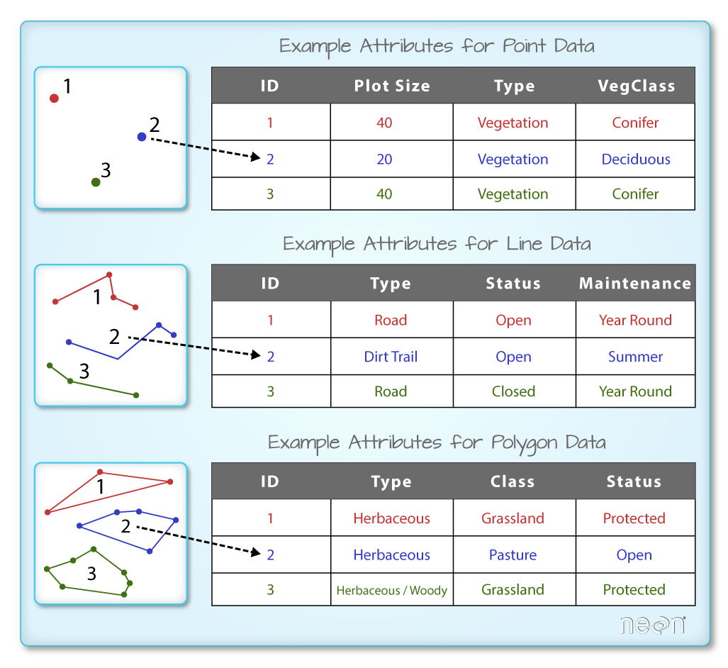
Figure 7.1: Geometry (left) and non-spatial attributes (right) of vector layers (https://www.neonscience.org/dc-shapefile-attributes-r)
7.1.2 Vector file formats
Commonly used vector layer file formats (Table 7.1) include binary formats (such as the Shapefile) and plain text formats (such as GeoJSON). Vector layers are also frequently kept in a spatial database, such as PostgreSQL/PostGIS.
| Type | Format | File extension |
|---|---|---|
| Binary | ESRI Shapefile | .shp, .shx, .dbf, .prj, … |
| GeoPackage (GPKG) | .gpkg |
|
| Plain Text | GeoJSON | .json or .geojson |
| GPS Exchange Format (GPX) | .gpx |
|
| Keyhole Markup Language (KML) | .kml |
|
| Spatial Databases | PostGIS / PostgreSQL |
7.1.3 The sp package
The first R package to establish a uniform vector layer class system was sp, released in 2005. Together with rgdal (2003) and rgeos (2011), the sp package dominated the landscape of spatial analysis in R for many years.
The sp package defines 6 main classes for vector layers (Table 7.2):
- One for each geometry type (points, lines, polygons)
- One for geometry only and one for geometry with attributes
| Class | Geometry type | Attributes |
|---|---|---|
SpatialPoints |
Points | - |
SpatialPointsDataFrame |
Points | data.frame |
SpatialLines |
Lines | - |
SpatialLinesDataFrame |
Lines | data.frame |
SpatialPolygons |
Polygons | - |
SpatialPolygonsDataFrame |
Polygons | data.frame |
We are not going to use sp in this book, but the newer sf package (Section 7.1.4). However, if you are going to work with spatial data in R it is very likely you will encounter sp in forums, books, or other packages, so it is important to be aware of it.
7.1.4 The sf package
The sf package (Figure 7.2), released in 2016, is a newer package for working with vector layers in R, which we are going to use in this book. In recent years, sf has become the standard package for working with vector data in R, practically replacing sp, rgdal, and rgeos.
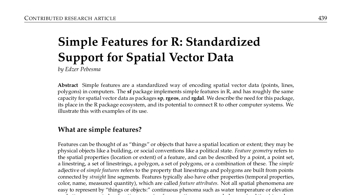
Figure 7.2: Pebesma, 2018, The R Journal (https://journal.r-project.org/archive/2018-1/)
One of the important innovations in sf is a complete implementation of the Simple Features standard. Since 2003, Simple Features been widely implemented in spatial databases (such as PostGIS), commercial GIS (e.g., ESRI ArcGIS) and forms the vector data basis for libraries such as GDAL. The Simple Features standard defines several types of geometries, of which seven are most commonly used in the world of GIS and spatial data analysis (Figure 7.6). When working with spatial databases, Simple Features are commonly specified as Well Known Text (WKT). A subset of simple features forms the GeoJSON standard.
The sf package depends on several external software components (installed along with the R package27), most importantly GDAL, GEOS and PROJ (Figure 7.3). These well-tested and popular open-source components are common to numerous open-source and commercial software for spatial analysis, such as QGIS and PostGIS.
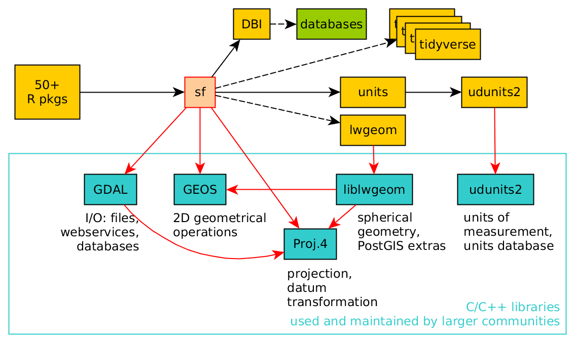
Figure 7.3: sf package dependencies (https://github.com/edzer/rstudio_conf)
Package sf defines a hierarchical class system with three classes (Table 7.3):
- Class
sfg—a single geometry - Class
sfc—a geometry column, which is a set ofsfggeometries + CRS information - Class
sf—a layer, which is ansfcgeometry column inside adata.framewith non-spatial attributes
| Class | Hierarchy | Information |
|---|---|---|
sfg |
Geometry | type, coordinates |
sfc |
Geometry column | set of sfg + CRS |
sf |
Layer | sfc + attributes |
The sf class represents a vector layer by extending the data.frame class, supplementing it with a geometry column. This is similar to the way that spatial databases are structured. For example, the sample dataset shown in Figure 7.4 represents a polygonal layer with three features and six non-spatial attributes. The attributes refer to demographic and epidemiological attributes of US counties, such as the number of births in 1974 (BIR74), the number of sudden infant death cases in 1974 (SID74), and so on. The seventh column is the geometry column, containing the polygon geometries.
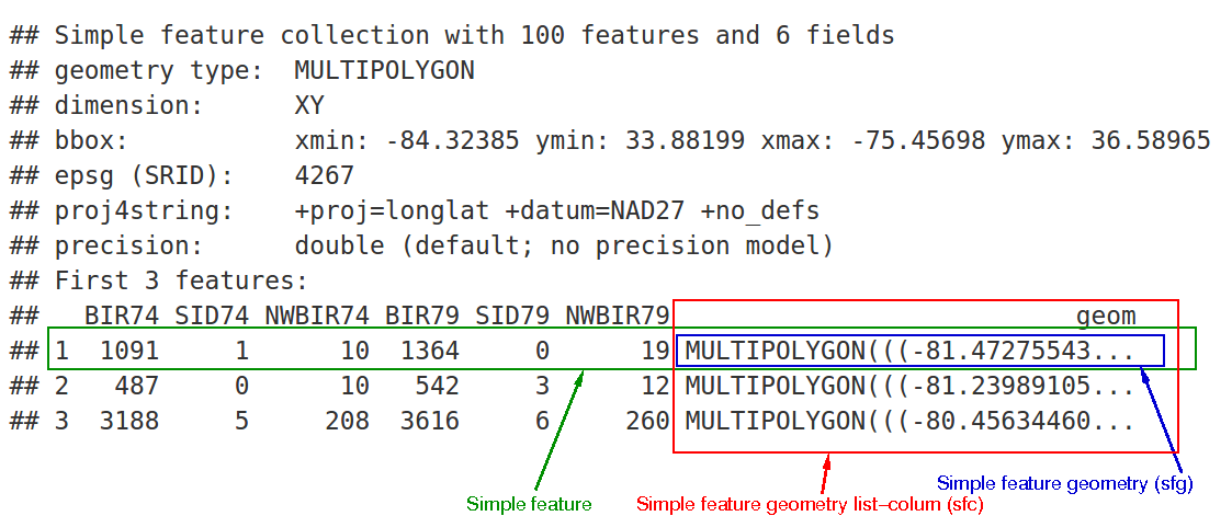
Figure 7.4: Structure of an sf object (https://cran.r-project.org/web/packages/sf/vignettes/sf1.html)
Figure 7.5 shows what the layer in Figure 7.4 would look like when mapped. We can see the outline of the three polygons, as well as the values of all six non-spatial attributes (in separate panels).
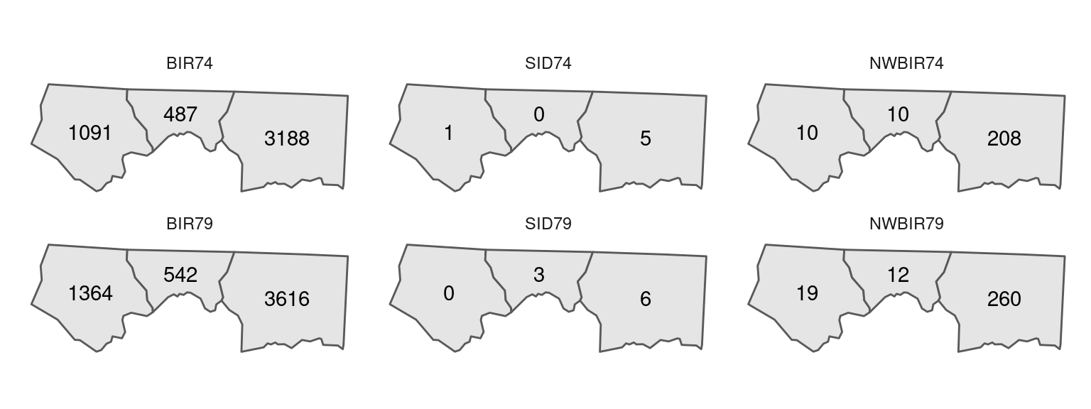
Figure 7.5: Visualization of the sf object shown in Figure 7.4
7.2 Vector layers from scratch
7.2.1 Overview
As mentioned above (Table 7.3), the sf package defines a hierarchical system of data structures, composed of three classes, from simple to complex: sfg, sfc and sf. In this section, we are going to create an object of each of those thress classes, to learn more about them.
7.2.2 Geometry (sfg)
Objects of class sfg, i.e., a single geometry, can be created using the appropriate function for each geometry type:
st_pointst_multipointst_linestringst_multilinestringst_polygonst_multipolygonst_geometrycollection
from coordinates passed as:
numericvectors—POINTmatrixobjects—MULTIPOINTorLINESTRINGlistobjects—All other geometries
The seven most commonly used Simple Feature geometry types are displayed in Figure 7.6.
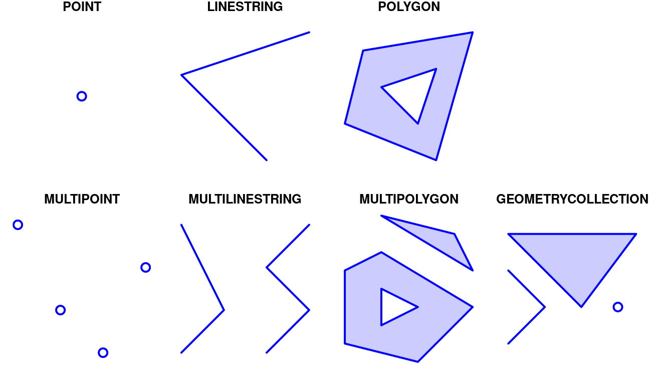
Figure 7.6: Simple feature geometry (sfg) types in package sf
Of those seven types, the GEOMETRYCOLLECTION is more rarely used and more difficult to work with. For example, the Shapefile format does not support geometries of type GEOMETRYCOLLECTION. You may wonder why does it even exist. One of the reasons is that some spatial operations may produce a mixture of geometry types. For example, the intersection (Section 8.3.4.6) between two polygons may be composed of points, lines, and polygons (Figure 7.7).
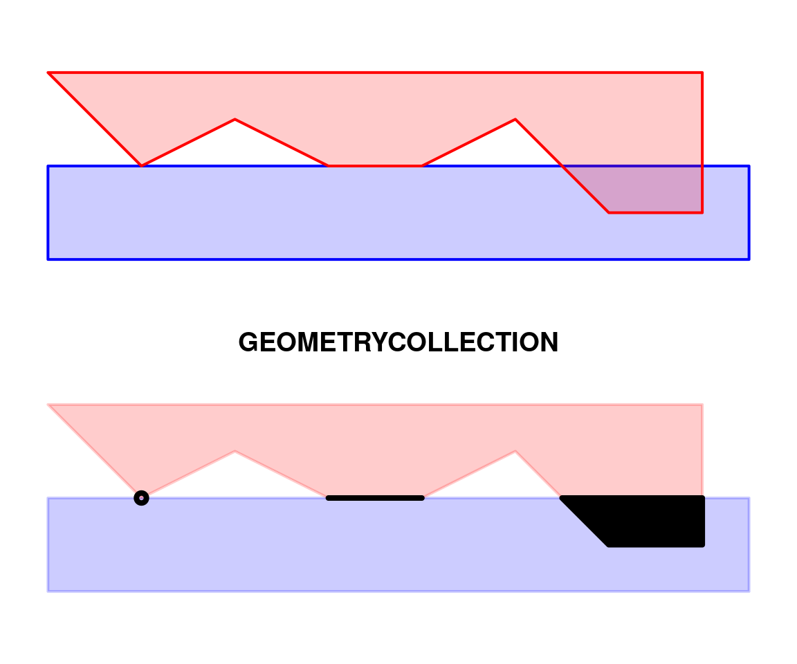
Figure 7.7: Intersection between two polygons may yield a GEOMETRYCOLLECTION
Let’s create some sfg geometries to see the principles in action. For example, we can create a point geometry object named pnt1, representing a POINT geometry, using the st_point function as follows:
library(sf)
pnt1 = st_point(c(34.798443, 31.243288))
Printing an sfg object in the console gives its WKT representation:
pnt1
## POINT (34.79844 31.24329)
Note that the class definition of an sfg (geometry) object:
class(pnt1)
## [1] "XY"    "POINT" "sfg"
is actually composed of three parts:
"XY"—The dimensions type (one of:"XY","XYZ","XYM"or"XYZM"). In this book, as in most cases of spatial analysis in general, we will be working only with two-dimensional"XY"geometries."POINT"—The geometry type (one of the geometry types:"POINT","MULTIPOINT", etc.)"sfg"—The general class (sfg= Simple Feature Geometry)
Here is another example of creating an sfg object. This time, we are creating a POLYGON geometry named a, using function st_polygon. (Don’t worry if the expression is unclear: we learn about using list in Chapter 11).
a = st_polygon(list(cbind(c(0,0,7.5,7.5,0),c(0,-1,-1,0,0))))Again, printing the object shows its WKT representation:
a
## POLYGON ((0 0, 0 -1, 7.5 -1, 7.5 0, 0 0))
while class reports the dimensionality, geometry type, and general class, in that order:
class(a)
## [1] "XY"      "POLYGON" "sfg"
The polygon is displayed in Figure 7.8:
plot(a, border = "blue", col = "#0000FF33", lwd = 2)
Figure 7.8: An sfg object of type POLYGON
Let’s create another POLYGON, named b:
b = st_polygon(list(cbind(c(0,1,2,3,4,5,6,7,7,0),c(1,0,0.5,0,0,0.5,-0.5,-0.5,1,1))))b
## POLYGON ((0 1, 1 0, 2 0.5, 3 0, 4 0, 5 0.5, 6 -0.5, 7 -0.5, 7 1, 0 1))class(b)
## [1] "XY" "POLYGON" "sfg"The second polygon is shown in Figure 7.9.
plot(b, border = "red", col = "#FF000033", lwd = 2)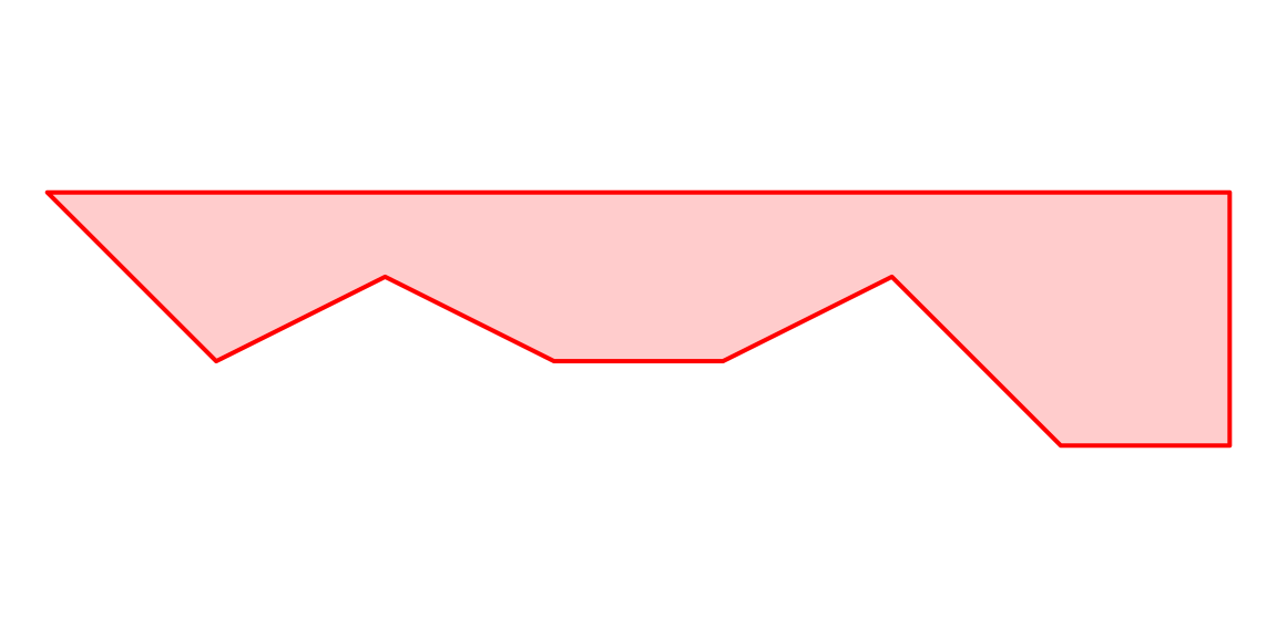
Figure 7.9: Another sfg object of type POLYGON
The c function, when given sfg geometries, combines those geometries into one. For example, combining two POLYGON geometries results in a single MULTIPOLYGON geometry:
ab = c(a, b)ab
## MULTIPOLYGON (((0 0, 0 -1, 7.5 -1, 7.5 0, 0 0)), ((0 1, 1 0, 2 0.5, 3 0, 4 0, 5 0.5, 6 -0.5, 7 -0.5, 7 1, 0 1)))class(ab)
## [1] "XY" "MULTIPOLYGON" "sfg"What type of geometry do you think
c(a, b, pnt1)is?
Keep in mind that c always returns a single geometry, composed of all the shapes in its input. This is different from collecting the geometries into a geometry column, where the geometries are kept separate, which is done using function st_sfc as shown below (Section 7.2.3).
The multipolygon we created is shown in Figure 7.10:
plot(ab, border = "darkgreen", col = "#00FF0033", lwd = 2)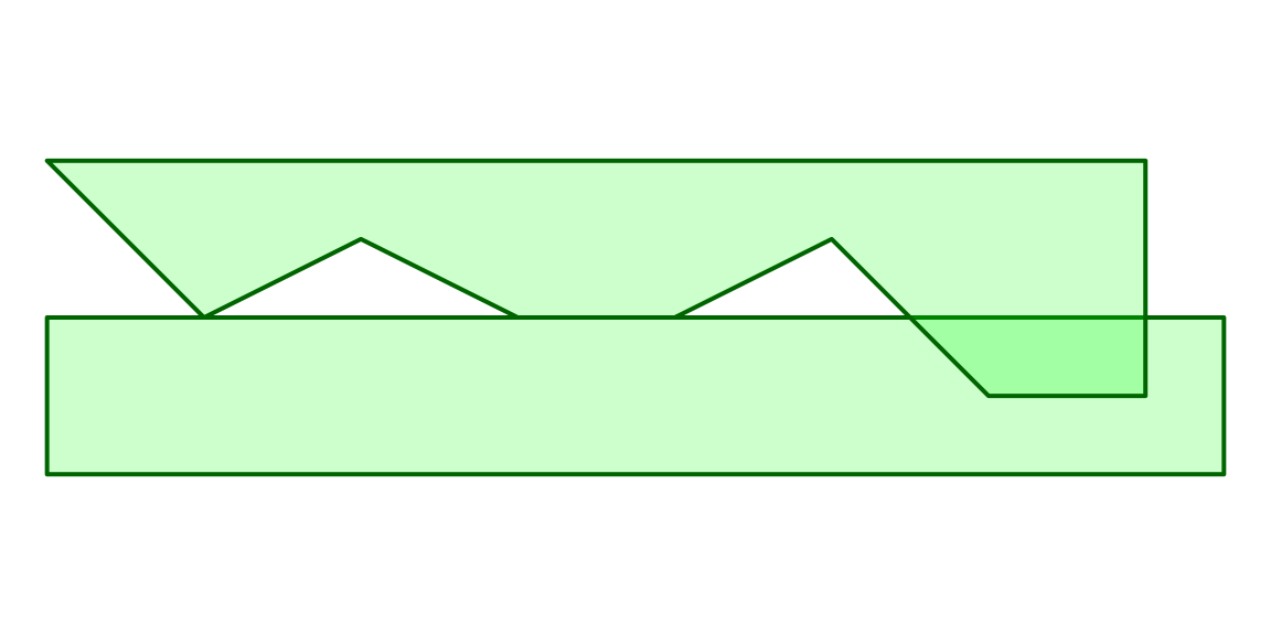
Figure 7.10: An sfg object of type MULTIPOLYGON
A new geometry can be calculated applying various functions on an existing one(s). For example, the following example calculates the intersection of a and b, which is a new geometry hereby named i. We are going to learn about st_intersection, and other geometry-generating functions, in Chapter 8.
i = st_intersection(a, b)The result happens to be a GEOMETRYCOLLECTION, as demonstrated in Figure 7.7:
i
## GEOMETRYCOLLECTION (POINT (1 0), LINESTRING (4 0, 3 0), POLYGON ((5.5 0, 7 0, 7 -0.5, 6 -0.5, 5.5 0)))class(i)
## [1] "XY" "GEOMETRYCOLLECTION" "sfg"Figure 7.11 displays the GEOMETRYCOLLECTION named i:
plot(i, border = "black", col = "darkgrey", lwd = 2)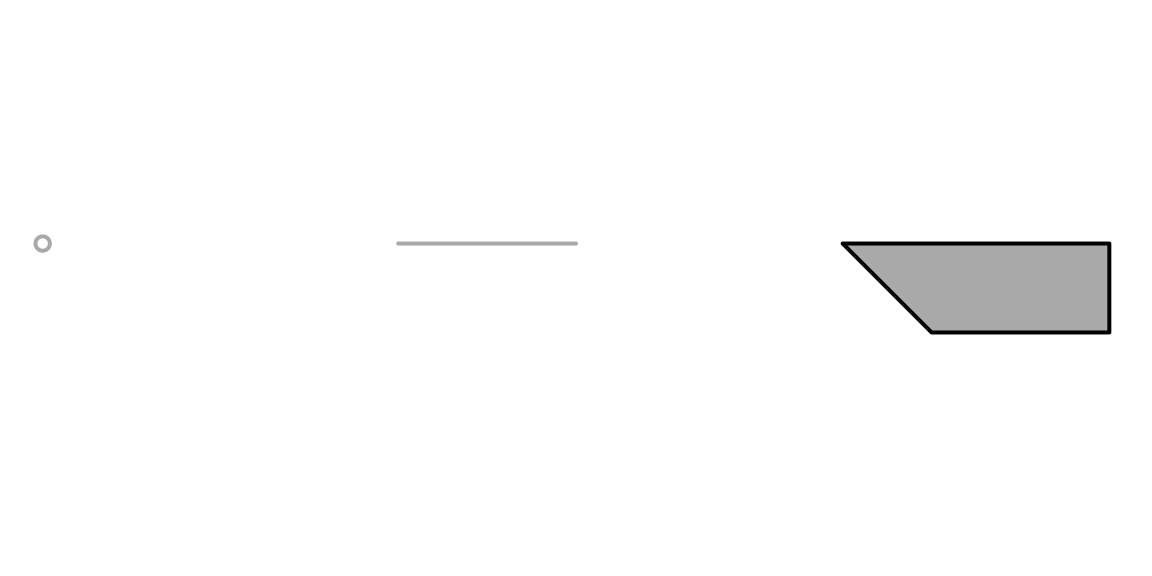
Figure 7.11: An sfg object of type GEOMETRYCOLLECTION
7.2.3 Geometry column (sfc)
Let’s create two more point geometries (Section 7.2.2) named pnt2 and pnt3, representing two more points:
pnt2 = st_point(c(34.812831, 31.260284))
pnt3 = st_point(c(35.011635, 31.068616))
Geometry objects (sfg) can be collected into a geometry column (sfc) object. This is done with function st_sfc.
In addition to the geometries, a geometry column object also contains a Coordinate Reference System (CRS) (more information on CRS is given below, in Section 7.9) definition, specified with the crs parameter of function st_sfc. Four types of CRS definitions are accepted:
- An EPSG code (e.g.,
4326) - A PROJ4 string (e.g.,
"+proj=longlat +datum=WGS84 +no_defs") - A WKT string
- A
crsobject of another layer, as returned byst_crs
Let’s combine the three POINT geometries—pnt1, pnt2 and pnt3—into a geometry column (sfc) object named geom. We will specify that the coordinates are lon/lat (WGS84), using the simplest of the three methods—an EPSG code (4326). More information on types of CRS, as well as where we can find the EPSG code of a particular CRS, is given in Section 7.9.2.
geom = st_sfc(pnt1, pnt2, pnt3, crs = 4326)Here is a summary of the resulting geometry column:
geom
## Geometry set for 3 features
## Geometry type: POINT
## Dimension:     XY
## Bounding box:  xmin: 34.79844 ymin: 31.06862 xmax: 35.01164 ymax: 31.26028
## Geodetic CRS:  WGS 84
## POINT (34.79844 31.24329)
## POINT (34.81283 31.26028)
## POINT (35.01163 31.06862)
The printout demostrates that other than the geometries themselves, and the derived properties of type, dimensionality, and bounding box, the geometry column contains the additional piece of information on the CRS.
7.2.4 Layer (sf)
A geometry column (sfc) can be combined with non-spatial columns, also known as attributes, resulting in a layer (sf) object. In our case, the three points in the sfc geometry column geom (Section 7.2.3) represent the location of the three railway stations in Beer-Sheva and Dimona. Let’s create a data.frame with several non-spatial properties of the stations, which we already worked with in Section 4.1.2, using function data.frame (Section 4.1.2):
name = c("Beer-Sheva Center", "Beer-Sheva University", "Dimona")
city = c("Beer-Sheva", "Beer-Sheva", "Dimona")
lines = c(4, 5, 1)
piano = c(FALSE, TRUE, FALSE)
dat = data.frame(name, city, lines, piano)
dat
##                    name       city lines piano
## 1     Beer-Sheva Center Beer-Sheva     4 FALSE
## 2 Beer-Sheva University Beer-Sheva     5  TRUE
## 3                Dimona     Dimona     1 FALSE
Note that the order of rows in the attribute table must match the order of the geometries!
dat
##                    name       city lines piano
## 1     Beer-Sheva Center Beer-Sheva     4 FALSE
## 2 Beer-Sheva University Beer-Sheva     5  TRUE
## 3                Dimona     Dimona     1 FALSE
Now, we can combine the attribute table dat (data.frame) and the geometry column geom (sfc). This is done using function st_sf, resulting in a layer (sf):
layer = st_sf(dat, geom)layer
## Simple feature collection with 3 features and 4 fields
## Geometry type: POINT
## Dimension: XY
## Bounding box: xmin: 34.79844 ymin: 31.06862 xmax: 35.01164 ymax: 31.26028
## Geodetic CRS: WGS 84
## name city lines piano geom
## 1 Beer-Sheva Center Beer-Sheva 4 FALSE POINT (34.79844 31.24329)
## 2 Beer-Sheva University Beer-Sheva 5 TRUE POINT (34.81283 31.26028)
## 3 Dimona Dimona 1 FALSE POINT (35.01163 31.06862)7.2.5 Interactive mapping with mapview
Function mapview—which we are familiar with from Section 5.3.7.2—is useful for inspecting vector layers too. For example:
library(mapview)
mapview(layer)
7.3 Extracting layer components
In Section 7.2 we:
- Started from raw coordinates
- Convered them to geometry objects (
sfg) using a function such asst_point,st_polygon, etc. (Section 7.2.2) - Combined the geometries to a geometry column (
sfc) using functionst_sfc(Section 7.2.3) - Added attributes to the geometry column to get a layer (
sf) using functionst_sf(Section 7.2.4)
which can be summarized as: coordinates → sfg → sfc → sf.
Sometimes we are interested in the opposite “direction.” In other words, we sometimes need to extract the simpler components (geometry, attributes, coordinates) from an existing layer:
sf→ geometry column (sfc)sf→ attribute table (data.frame)sf→ coordinates (matrix)
The geometry column (sfc) component can be extracted from an sf layer object using function st_geometry:
st_geometry(layer)
## Geometry set for 3 features
## Geometry type: POINT
## Dimension:     XY
## Bounding box:  xmin: 34.79844 ymin: 31.06862 xmax: 35.01164 ymax: 31.26028
## Geodetic CRS:  WGS 84
## POINT (34.79844 31.24329)
## POINT (34.81283 31.26028)
## POINT (35.01163 31.06862)
The non-spatial columns of an sf layer, i.e., the attribute table, can be extracted from an sf object using function st_drop_geometry:
st_drop_geometry(layer)
##                    name       city lines piano
## 1     Beer-Sheva Center Beer-Sheva     4 FALSE
## 2 Beer-Sheva University Beer-Sheva     5  TRUE
## 3                Dimona     Dimona     1 FALSE
The latter is analogous to opening an attribute table of a vector layer in GIS software, such as ArcGIS (Figure 7.12).
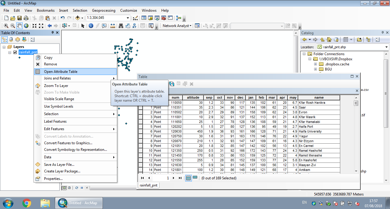
Figure 7.12: Attribute table in ArcGIS
The coordinates of sf, sfc or sfg objects can be obtained with function st_coordinates. The coordinates are returned as a matrix:
st_coordinates(layer)
##          X        Y
## 1 34.79844 31.24329
## 2 34.81283 31.26028
## 3 35.01163 31.06862
In the case of a two-dimensional POINT layer, which is the most common use case of st_coordinates, the returned matrix has two columns X and Y as shown above. (With other types of geometries, the matrix has additional columns containing the information on grouping of point coordinates into shapes.)
7.4 Creating point layer from table
A common way of creating a point layer is to transform a table which has X and Y coordinate columns. Function st_as_sf can transform a table (data.frame) into a point layer (sf). In st_as_sf we specify:
x—Thedata.frameto be convertedcoords—Columns names with the coordinates (X, Y)crs—The CRS (NAif left unspecified)
Let’s take the rainfall.csv table as an example. This table contains UTM 36N (EPSG: 32636) coordinates in the columns named x_utm and y_utm:
rainfall = read.csv("rainfall.csv")head(rainfall)
## num altitude sep oct nov dec jan feb mar apr may name
## 1 110050 30 1.2 33 90 117 135 102 61 20 6.7 Kfar Rosh Hanikra
## 2 110351 35 2.3 34 86 121 144 106 62 23 4.5 Saar
## 3 110502 20 2.7 29 89 131 158 109 62 24 3.8 Evron
## 4 111001 10 2.9 32 91 137 152 113 61 21 4.8 Kfar Masrik
## 5 111650 25 1.0 27 78 128 136 108 59 21 4.7 Kfar Hamakabi
## 6 120202 5 1.5 27 80 127 136 95 49 19 2.7 Haifa Port
## x_utm y_utm
## 1 696533.1 3660837
## 2 697119.1 3656748
## 3 696509.3 3652434
## 4 696541.7 3641332
## 5 697875.3 3630156
## 6 687006.2 3633330The table can be converted to an sf layer using st_as_sf as follows:
rainfall = st_as_sf(rainfall, coords = c("x_utm", "y_utm"), crs = 32636)Note:
- The order of
coordscolumn names corresponds to X-Y! 32636is the EPSG code of the UTM 36N projection (Table 7.4)
The analogous operation in ArcGIS is the Display XY Data menu (Figures 7.13–7.15).
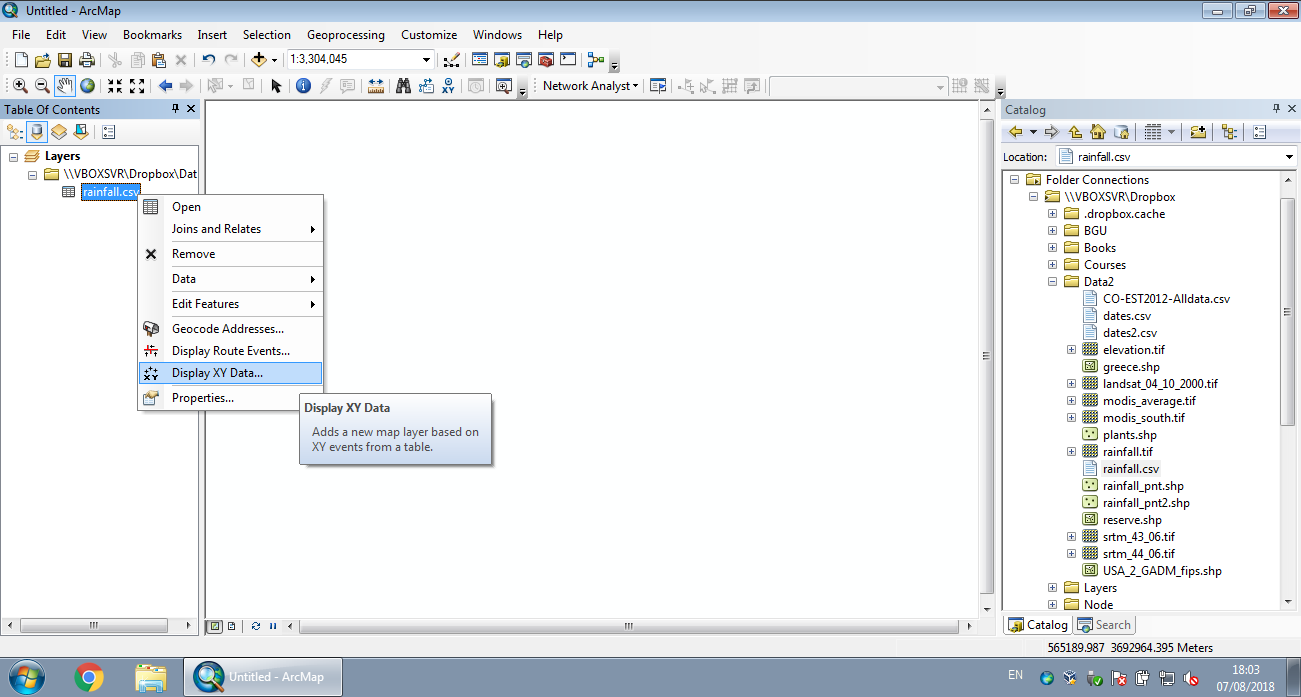
Figure 7.13: Displaying XY data from CSV in ArcGIS (Step 1)
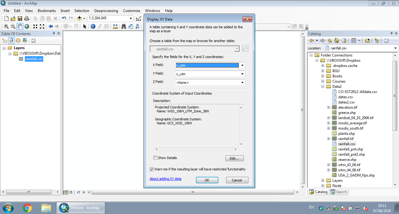
Figure 7.14: Displaying XY data from CSV in ArcGIS (Step 2)
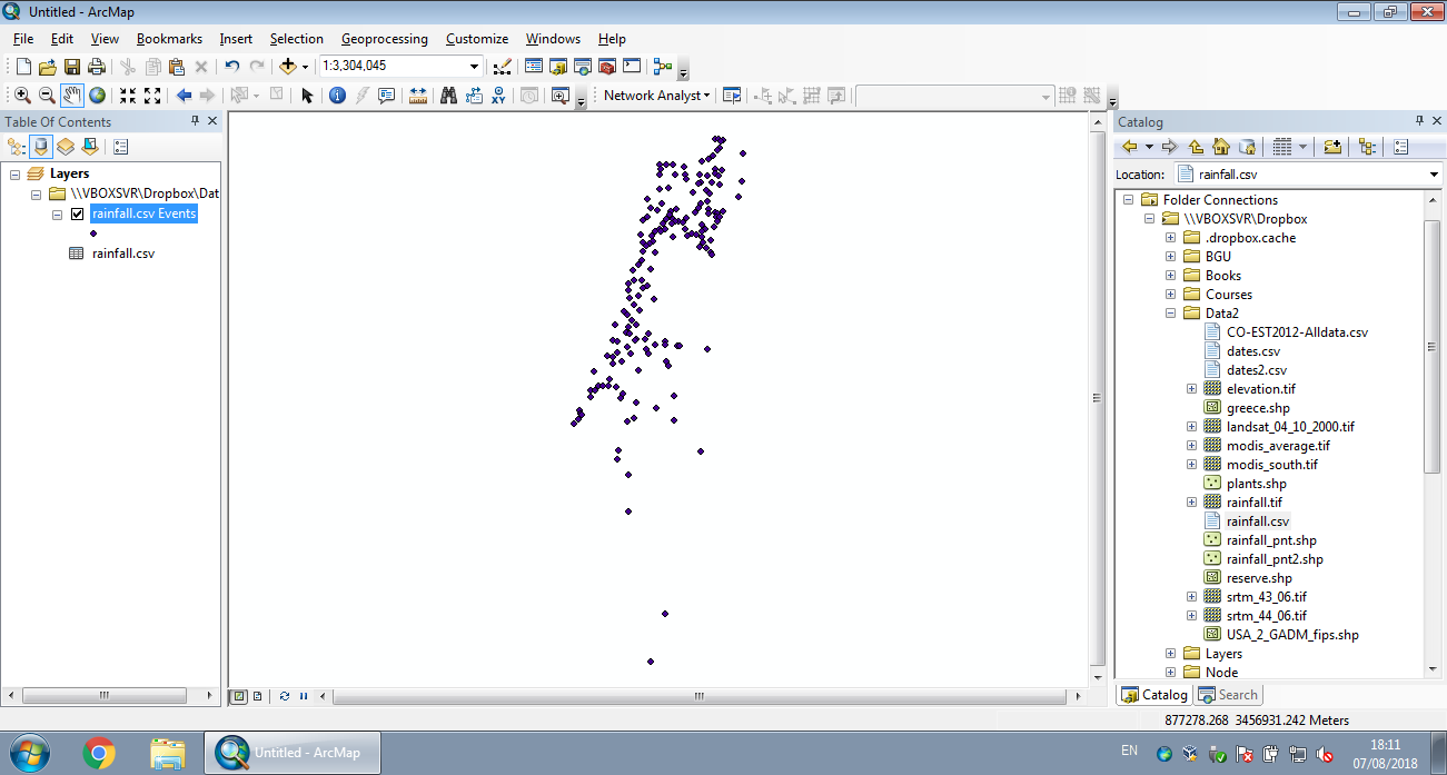
Figure 7.15: Displaying XY data from CSV in ArcGIS (Step 3)
Here is the resulting sf layer:
rainfall
## Simple feature collection with 169 features and 12 fields
## Geometry type: POINT
## Dimension:     XY
## Bounding box:  xmin: 629301.4 ymin: 3270290 xmax: 761589.2 ymax: 3681163
## Projected CRS: WGS 84 / UTM zone 36N
## First 10 features:
##       num altitude sep oct nov dec jan feb mar apr may              name
## 1  110050       30 1.2  33  90 117 135 102  61  20 6.7 Kfar Rosh Hanikra
## 2  110351       35 2.3  34  86 121 144 106  62  23 4.5              Saar
## 3  110502       20 2.7  29  89 131 158 109  62  24 3.8             Evron
## 4  111001       10 2.9  32  91 137 152 113  61  21 4.8       Kfar Masrik
## 5  111650       25 1.0  27  78 128 136 108  59  21 4.7     Kfar Hamakabi
## 6  120202        5 1.5  27  80 127 136  95  49  19 2.7        Haifa Port
## 7  120630      450 1.9  36  93 161 166 128  71  21 4.9  Haifa University
## 8  120750       30 1.6  31  91 163 170 146  76  22 4.9             Yagur
## 9  120870      210 1.1  32  93 147 147 109  61  16 4.3        Nir Etzyon
## 10 121051       20 1.8  32  85 147 142 102  56  13 4.5         En Carmel
##                    geometry
## 1  POINT (696533.1 3660837)
## 2  POINT (697119.1 3656748)
## 3  POINT (696509.3 3652434)
## 4  POINT (696541.7 3641332)
## 5  POINT (697875.3 3630156)
## 6  POINT (687006.2 3633330)
## 7  POINT (689553.7 3626282)
## 8  POINT (694694.5 3624388)
## 9  POINT (686489.5 3619716)
## 10 POINT (683148.4 3616846)
An interactive map, showing the spatial locations of the rainfall stations, can be created using mapview (Section 7.2.5). Here, we are using the additional zcol parameter to choose which attribute will be used for the color scale:
mapview(rainfall, zcol = "jan")7.5 sf layer properties
7.5.1 Dimensions
An sf layer is basically a special type of data.frame, where one of the columns is a geometry column. Therefore, many of the functions we learned when working with data.frame tables (Chapter 4) also work on sf layers.
For example, we can get the number of rows, or features, with nrow:
nrow(rainfall)
## [1] 169
and the number of columns (including the geometry column) with ncol:
ncol(rainfall)
## [1] 13
or both with dim:
dim(rainfall)
## [1] 169  13
What is the result of
st_geometry(rainfall)?st_drop_geometry(rainfall)?
7.5.2 Spatial properties
The st_bbox function returns the bounding box coordinates, just like for stars objects (Section 5.3.8.3):
st_bbox(rainfall)
##      xmin      ymin      xmax      ymax
##  629301.4 3270290.2  761589.2 3681162.7
The st_crs function returns the Coordinate Reference System (CRS), also the same way as for stars objects (Section 5.3.8.3):
st_crs(rainfall)
## Coordinate Reference System:
##   User input: EPSG:32636
##   wkt:
## PROJCRS["WGS 84 / UTM zone 36N",
##     BASEGEOGCRS["WGS 84",
##         DATUM["World Geodetic System 1984",
##             ELLIPSOID["WGS 84",6378137,298.257223563,
##                 LENGTHUNIT["metre",1]]],
##         PRIMEM["Greenwich",0,
##             ANGLEUNIT["degree",0.0174532925199433]],
##         ID["EPSG",4326]],
##     CONVERSION["UTM zone 36N",
##         METHOD["Transverse Mercator",
##             ID["EPSG",9807]],
##         PARAMETER["Latitude of natural origin",0,
##             ANGLEUNIT["degree",0.0174532925199433],
##             ID["EPSG",8801]],
##         PARAMETER["Longitude of natural origin",33,
##             ANGLEUNIT["degree",0.0174532925199433],
##             ID["EPSG",8802]],
##         PARAMETER["Scale factor at natural origin",0.9996,
##             SCALEUNIT["unity",1],
##             ID["EPSG",8805]],
##         PARAMETER["False easting",500000,
##             LENGTHUNIT["metre",1],
##             ID["EPSG",8806]],
##         PARAMETER["False northing",0,
##             LENGTHUNIT["metre",1],
##             ID["EPSG",8807]]],
##     CS[Cartesian,2],
##         AXIS["(E)",east,
##             ORDER[1],
##             LENGTHUNIT["metre",1]],
##         AXIS["(N)",north,
##             ORDER[2],
##             LENGTHUNIT["metre",1]],
##     USAGE[
##         SCOPE["unknown"],
##         AREA["World - N hemisphere - 30°E to 36°E - by country"],
##         BBOX[0,30,84,36]],
##     ID["EPSG",32636]]
Question: what is the difference between the two plots in Figure 7.16, created using the following expressions?
plot(st_geometry(rainfall))
plot(st_coordinates(rainfall)[, 1], st_coordinates(rainfall)[, 2])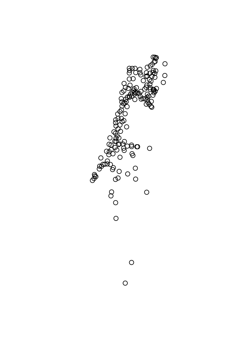
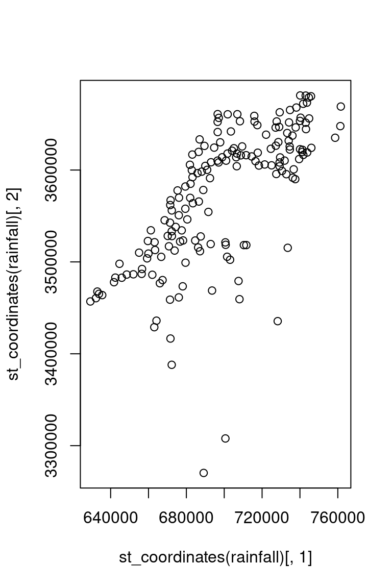
Figure 7.16: Two plots
7.6 Subsetting based on attributes
Subsetting of features in an sf vector layer is exactly the same as filtering rows in a data.frame (Section 4.1.5). Remember: an sf layer is a data.frame. For example, the following expressions subset the rainfall layer:
rainfall[1:10, ]
rainfall[rainfall$jan > 100, ]
Which meteorological stations are being selected in each of these two expressions?
Figure 7.17 shows the resulting subsets:
plot(st_geometry(rainfall[1:10, ]), main = "rainfall[1:10, ]")
plot(st_geometry(rainfall[rainfall$jan > 100, ]), main = "rainfall[rainfall$jan > 100, ]")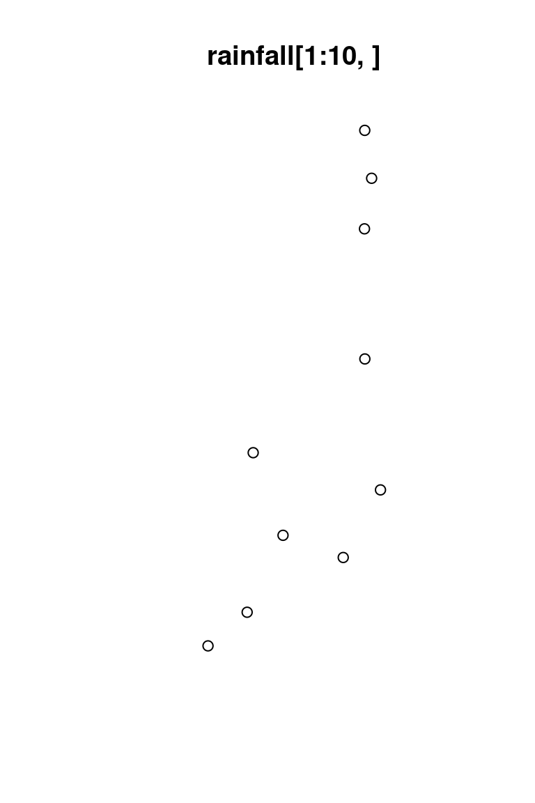
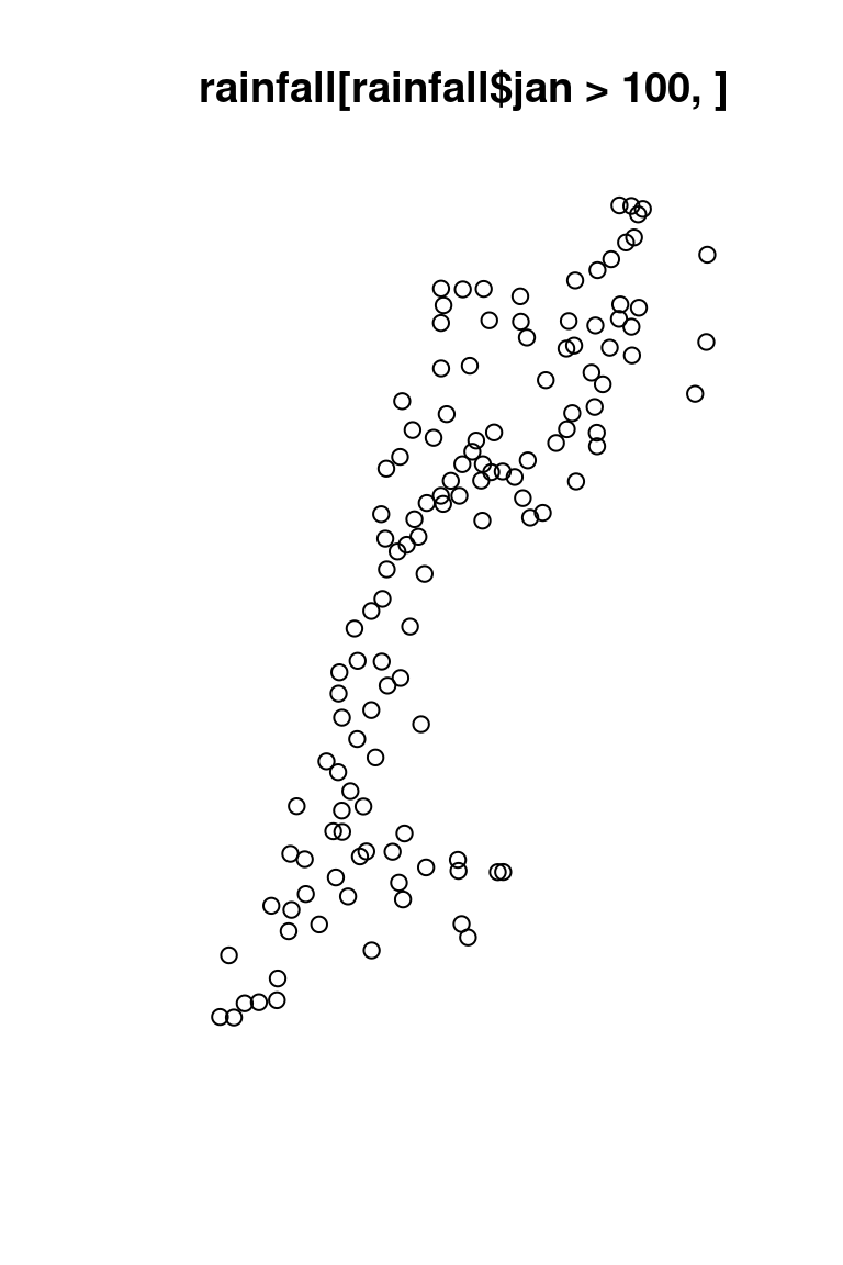
Figure 7.17: Subsets of the rainfall layer
Subsetting columns in sf is also similar to subsetting columns in a data.frame, with one exception: the geometry column. The geometry column “sticks” to the subset, by default, even if we do not explicitly select it, so that the resulting subset remains an sf object:
rainfall[1:5, c("jan", "feb")]
## Simple feature collection with 5 features and 2 fields
## Geometry type: POINT
## Dimension:     XY
## Bounding box:  xmin: 696509.3 ymin: 3630156 xmax: 697875.3 ymax: 3660837
## Projected CRS: WGS 84 / UTM zone 36N
##   jan feb                 geometry
## 1 135 102 POINT (696533.1 3660837)
## 2 144 106 POINT (697119.1 3656748)
## 3 158 109 POINT (696509.3 3652434)
## 4 152 113 POINT (696541.7 3641332)
## 5 136 108 POINT (697875.3 3630156)
In case we do need to omit the geometry column and get a data.frame, we can apply st_drop_geometry (Section 7.3) on the subset:
st_drop_geometry(rainfall[1:5, c("jan", "feb")])
##   jan feb
## 1 135 102
## 2 144 106
## 3 158 109
## 4 152 113
## 5 136 108
7.7 Reading vector layers
In addition to creating from raw coordinates (Section 7.2) and transforming a data.frame to point layer (Section 7.4), we often create vector layers by reading from a file or from a spatial database (Section 7.1.2)28. Reading a vector layer from a file or a database is done using the st_read function.
For example, the following expression reads the Shapefile of US county boundaries, named USA_2_GADM_fips.shp, from the course materials. In case the Shapefile is located in the working directory, we need to specify the name of just the .shp file, even though the Shapefile contains several other files (Table 7.1):
county = st_read("USA_2_GADM_fips.shp")county
## Simple feature collection with 3103 features and 4 fields
## Geometry type: MULTIPOLYGON
## Dimension: XY
## Bounding box: xmin: -124.7628 ymin: 24.52042 xmax: -66.94889 ymax: 49.3833
## Geodetic CRS: WGS 84
## First 10 features:
## NAME_1 NAME_2 TYPE_2 FIPS geometry
## 1 Connecticut Litchfield County 09005 MULTIPOLYGON (((-73.05166 4...
## 2 Connecticut Hartford County 09003 MULTIPOLYGON (((-72.50941 4...
## 3 Connecticut Tolland County 09013 MULTIPOLYGON (((-72.13582 4...
## 4 Connecticut Windham County 09015 MULTIPOLYGON (((-71.79794 4...
## 5 California Siskiyou County 06093 MULTIPOLYGON (((-122.2873 4...
## 6 California Del Norte County 06015 MULTIPOLYGON (((-124.2492 4...
## 7 California Modoc County 06049 MULTIPOLYGON (((-120.0003 4...
## 8 Connecticut New London County 09011 MULTIPOLYGON (((-72.225 41....
## 9 Connecticut Fairfield County 09001 MULTIPOLYGON (((-73.65778 4...
## 10 Connecticut Middlesex County 09007 MULTIPOLYGON (((-72.47361 4...Let’s also read a GeoJSON file with the location of three particular airports in New Mexico:
airports = st_read("airports.geojson")airports
## Simple feature collection with 3 features and 1 field
## Geometry type: POINT
## Dimension: XY
## Bounding box: xmin: -106.7947 ymin: 35.04807 xmax: -106.0892 ymax: 35.61621
## Geodetic CRS: WGS 84
## name geometry
## 1 Albuquerque International POINT (-106.6169 35.04807)
## 2 Double Eagle II POINT (-106.7947 35.15559)
## 3 Santa Fe Municipal POINT (-106.0892 35.61621)7.8 Basic plotting
When plotting an sf object with plot, we get multiple small maps—one map for each attribute. This can be useful to quickly examine the types of spatial variation in our data. For example (Figure 7.18):
plot(county)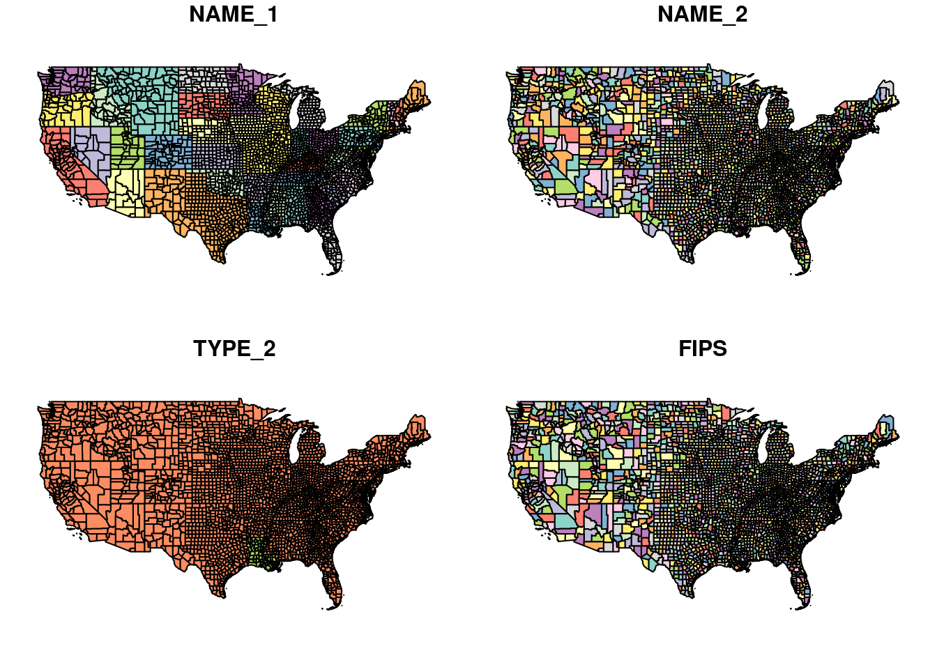
Figure 7.18: Plot of sf object
Plotting a single attribute adds a legend (Figure 7.19). The key.width and key.pos let us control the amount of space the legend takes and its placement, respectively:
plot(county[, "TYPE_2"], key.width = lcm(5), key.pos = 4)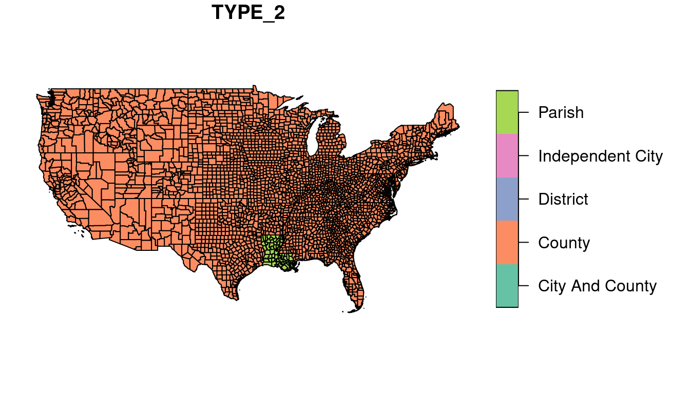
Figure 7.19: Plot of sf object, single attribute with legend
Plotting an sfc or an sfg object shows just the geometry (Figure 7.20):
plot(st_geometry(county))
Figure 7.20: Plot of sfc object
We can use graphical parameters to control the appearance of plotted geometries, such as:
col—Fill colorborder—Outline colorpch—Point shapecex—Point size
For example, the following expression draws county borders in grey (Figure 7.21):
plot(st_geometry(county), border = "grey")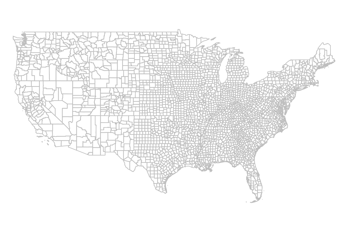
Figure 7.21: Basic plot of sfc object
Additional vector layers can be drawn in an existing graphical window using add=TRUE, similarly to the concept of layers in GIS software. For example, the following expressions draw both county and airports geometries (Figure 7.22). Note how the second expression uses add=TRUE:
plot(st_geometry(county), border = "grey")
plot(st_geometry(airports), col = "red", add = TRUE)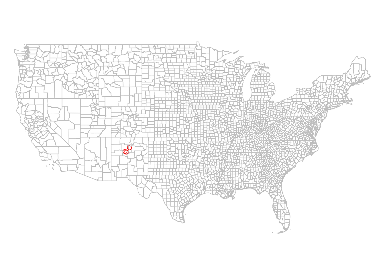
Figure 7.22: Using add=TRUE in plot
We can also use add=TRUE to combine sfg or sfc geometries with rasters in the same plot. For example, let’s plot the rainfall layer on top of the rainfall.tif raster, which is an interpolated rainfall surface we met in Chapter 1. First we will read the raster file:
library(stars)
r = read_stars("rainfall.tif")
names(r) = "rainfall (mm)"
and then plot both layers (Figure 7.23):
plot(r, breaks = "equal", col = hcl.colors(11, "Spectral"), reset = FALSE)
plot(st_geometry(rainfall), add = TRUE)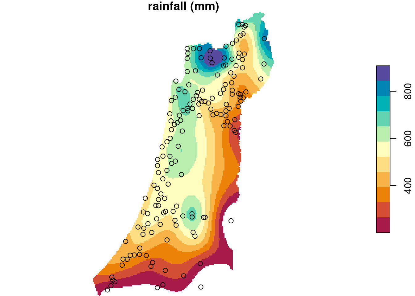
Figure 7.23: sfc layer on top of a raster
Note that we need to use the additional argument reset=FALSE whenever we are adding more layers to a stars raster plot.
7.9 Coordinate Reference Systems (CRS)
7.9.1 What are CRS?
A Coordinate Reference System (CRS) defines how the coordinates in our geometries relate to the surface of the Earth. There are two main types of CRS:
- Geographic—longitude and latitude, in degrees
- Projected—implying flat surface, usually in units of true distance (e.g., meters)
For example, Figure 7.24 shows the same polygonal layer (U.S. counties) in two different projection. On the left, the county layer is in the WGS84 geographic projection. Indeed, we can see that the axes are given in degrees of longitude and latitude. For example, we can see how the nothern border of U.S. follows the 49° latitude line. On the right, the same layer is displayed in the US National Atlas projection, where units are arbitrary but reflect true distance (meters). For example, the distance between every two consecutive grid lines is 1,000,000 meters or 1,000 kilometers.
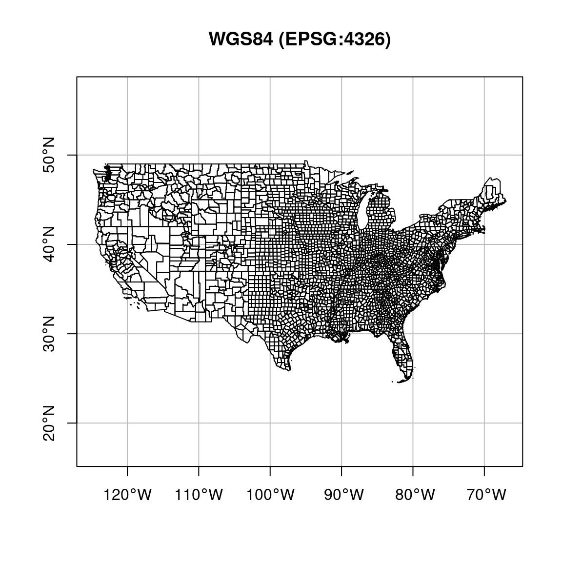
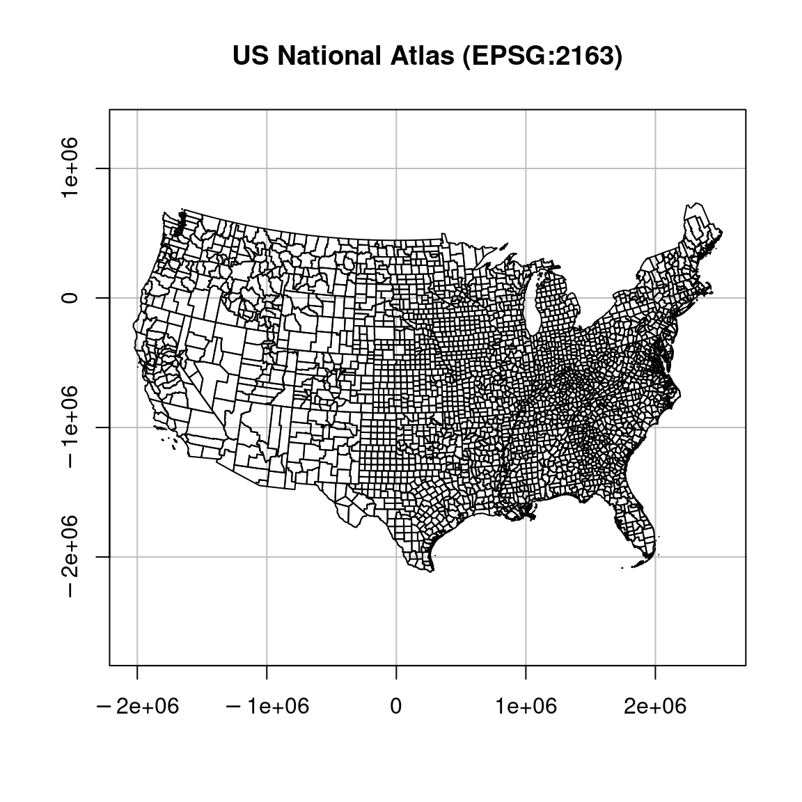
Figure 7.24: US counties in WGS84 and US Atlas projections
7.9.2 Vector layer reprojection
Reprojection is the transformation of geometry coordinates, from one CRS to another. It is an important part of spatial analysis workflow, since we often need to:
- Transform several layers into the same projection, so that they can be displayed one on top of the other (e.g., Figure 7.22) or so that they can be subject to a spatial operator (e.g., Figure 7.7)
- Switch between geographic and projected CRS
A vector layer can be reprojected with st_transform. The st_transform function has two important parameters:
x—The layer to be reprojectedcrs—The target CRS
Why don’t we need to specify the origin CRS in
st_transform?
As mentioned above, the CRS can be specified in one of four ways, using an EPSG code, a PROJ4 string, a WKT string, or a crs object (Section 7.2.3). Where can we find EPSG codes or WKT definitions of different projections?
- We can use CRS databases on the internet, such as http://spatialreference.org or http://epsg.io/, to look up CRS definitions for a given country, of CRS name, using the search box.
- We can use the
make_EPSGfunction from thergdalpackage in R, which returns adata.frameof CRS definitions. Thedata.framecan be filtered to locate the CRS of interest. For example, the following expressions return the information on CRS where the description contains the word “Israel.”
library(rgdal)
dat = make_EPSG()
dat[grepl("Israel", dat$note), ]
##       code                             note
## 86    4141                      Israel 1993
## 1158  2039    Israel 1993 / Israeli TM Grid
## 2527 28193 Palestine 1923 / Israeli CS Grid
## 5458  6984                  Israeli Grid 05
## 5459  6991               Israeli Grid 05/12
##                                                                                                                                                       prj4
## 86                                                                                                           +proj=longlat +ellps=GRS80 +no_defs +type=crs
## 1158      +proj=tmerc +lat_0=31.7343936111111 +lon_0=35.2045169444444 +k=1.0000067 +x_0=219529.584 +y_0=626907.39 +ellps=GRS80 +units=m +no_defs +type=crs
## 2527 +proj=cass +lat_0=31.7340969444444 +lon_0=35.2120805555556 +x_0=170251.555 +y_0=1126867.909 +a=6378300.789 +b=6356566.435 +units=m +no_defs +type=crs
## 5458      +proj=tmerc +lat_0=31.7343936111111 +lon_0=35.2045169444444 +k=1.0000067 +x_0=219529.584 +y_0=626907.39 +ellps=GRS80 +units=m +no_defs +type=crs
## 5459      +proj=tmerc +lat_0=31.7343936111111 +lon_0=35.2045169444444 +k=1.0000067 +x_0=219529.584 +y_0=626907.39 +ellps=GRS80 +units=m +no_defs +type=crs
##               prj_method
## 86                (null)
## 1158 Transverse Mercator
## 2527     Cassini-Soldner
## 5458 Transverse Mercator
## 5459 Transverse Mercator
In this book, we are going to encounter five different projections: WGS84, Sinusoidal, UTM 36N, ITM and US National Atlas (Table 7.4). We are going to specify them (e.g., in st_transform) using their EPSG codes, which is the easiest method.
| Name | Type | Area | Units | EPSG code |
|---|---|---|---|---|
| WGS84 | Geographic | World | degrees | 4326 |
| Sinusoidal | Projected | World | meters | - |
| UTM 36N | Projected | Israel | meters | 32636 |
| ITM | Projected | Israel | meters | 2039 |
| US National Atlas | Projected | USA | meters | 2163 |
Now, let’s see how we can use the st_transform function to repriject layers, in practice. The county and airports are currently in WGS84 (EPSG:4326) (How can we check?). Suppose that we would like to reproject those layers to the the US National Atlas Equal Area projection (EPSG:2163). The following expressions implement the reprojection:
county = st_transform(county, 2163)
airports = st_transform(airports, 2163)
The modified layers are shown in Figure 7.25. We can clearly see that the layer orientation has changes (also see Figure 7.24).
plot(st_geometry(county), border = "grey")
plot(st_geometry(airports), col = "red", add = TRUE)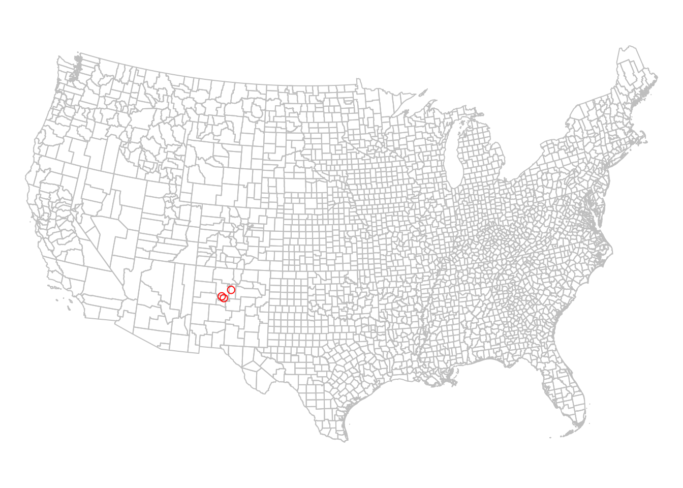
Figure 7.25: The county and airports layers in the US National Atlas Projection (EPSG=2163)
Examining the layer coordinates also shows that, indeed, the coordinates have changed with reprojecton:
st_coordinates(st_transform(airports, 4326))  # WGS84 coordinates
##           X        Y
## 1 -106.6169 35.04807
## 2 -106.7947 35.15559
## 3 -106.0892 35.61621st_coordinates(st_transform(airports, 2163)) # US National Atlas coordinates
## X Y
## 1 -603868.2 -1081605
## 2 -619184.5 -1068431
## 3 -551689.8 -1022366Create a subset of
countywith the counties of New-Mexico, Arizona and Texas only, and plot the result (Figure 7.26).
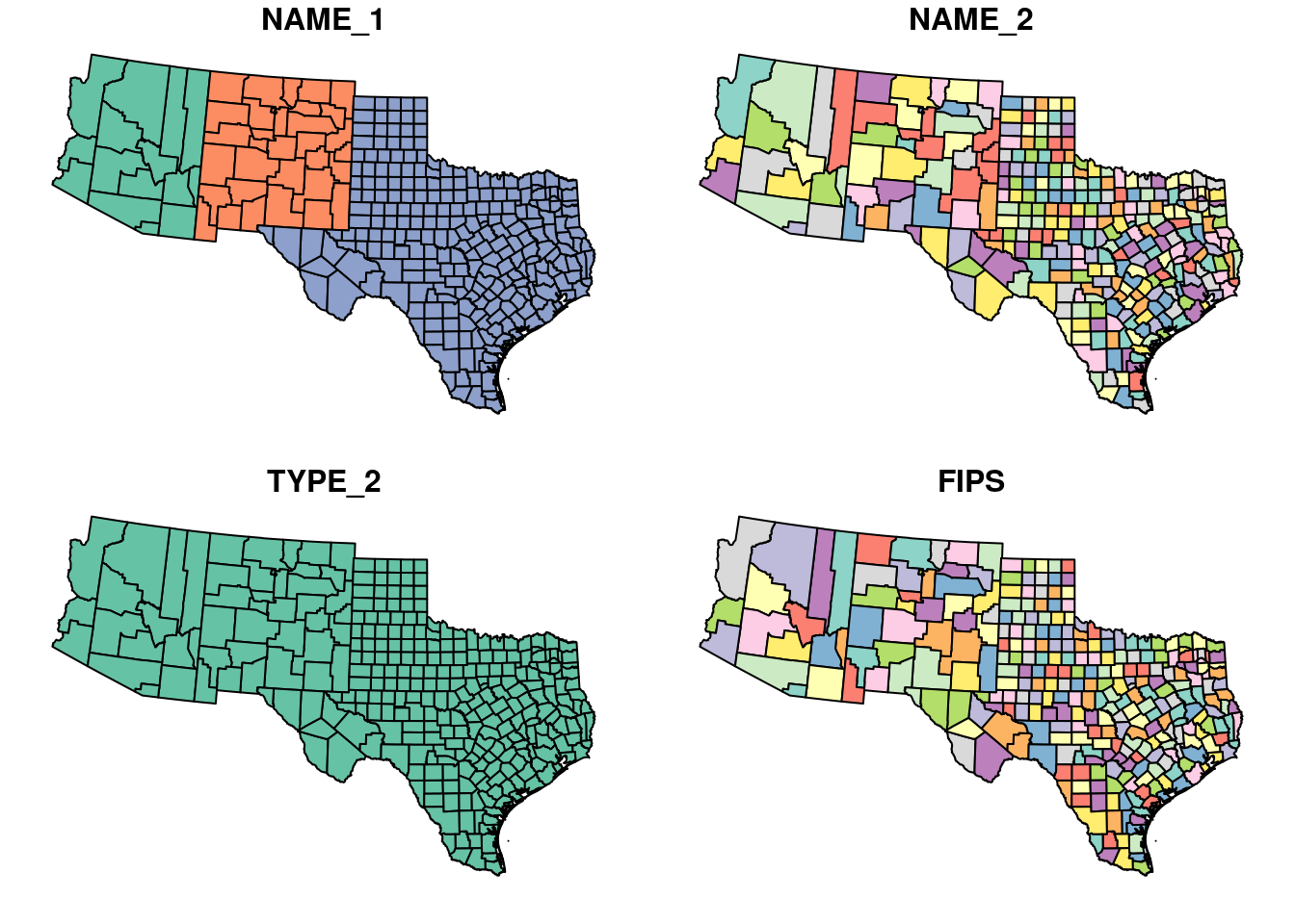
Figure 7.26: Subset of three states from the county layer
7.10 Writing vector layers
Writing an sf object to a file can be done with st_write. Before writing the rainfall layer to disk, let’s calculate a new column called annual with the annual rainfall (Section 4.5):
m = c("sep", "oct", "nov", "dec", "jan", "feb", "mar", "apr", "may")
rainfall$annual = apply(st_drop_geometry(rainfall[, m]), 1, sum)
In the last expression, why did we use
st_drop_geometry(rainfall[, m])as the first argument inapply, instead ofrainfall[, m]?
The sf object can be written to a Shapefile with st_write, as follows:
st_write(rainfall, "rainfall_pnt.shp")The format is automatically determined based on the .shp file extension. To overwrite an existing file, use delete_dsn=TRUE.