Vector layers (geopandas)

Last updated: 2023-02-25 13:40:03

---

Introduction

In the previous chapter, we worked with individual geometries using the shapely package (Geometries (shapely)). In GIS paractice, however, we usually work with vector layers, rather than individual geometries. Vector layers can be thought of:

• a collection of (one or more) geometries,

• associated with a Coordinate Reference System (CRS), and

• associated with (zero or more) non-spatial attributes.

In this chapter, we introduce the geopandas package for working with vector layers. First, we are going to see how a vector layer can be created from scratch (see Creating a GeoDataFrame), using shapely geometries, to understand the relation between shapely geometries and geopandas data structures, namely:

• GeoSeries—A geometry column, i.e., a collection of geometries along with a CRS definition

• GeoDataFrame—A vector layer

Then, we go on to cover some of the basic operations and workflows with vector layers using the geopandas package:

• Reading vector layers—Importing a vector layer from a file, such as a Shapefile

• Plotting (geopandas)—Plotting vector layers

• Filtering by attributes—Selecting features by attribute

• Table to point layer—Creating a point layer from a table

• Points to line (geopandas)—Converting a point layer to a line layer

• Writing vector layers—Writing a vector layer to file

In the next chapter, we are going to cover spatial operations with geopandas, such as calculating new geometries (buffers, etc.) and spatial join (see Geometric operations).

What is geopandas?

geopandas, as the name suggests, is an extension of pandas that enables working with spatial (geographic) data, specifically with vector layers. To facilitate the representation of spatial data, geopandas defines two data structures, which are extensions of the analogous data structures from pandas for non-spatial data:

• GeoSeries—An extension of a Series (see Creating a Series) for storing a sequence of geometries and a Coordinate Reference System (CRS) definition, whereas each geometry is a shapely object (see Geometries (shapely))

• GeoDataFrame—An extension of a DataFrame (see Creating a DataFrame), where one of the columns is a GeoSeries

As will be demostrated in a moment (see Creating a GeoDataFrame), a GeoDataFrame, representing a vector layer, is thus a combination (Fig. 47) of:

• A GeoSeries, which holds the geometries in a special “geometry” column

• Zero or more Series, which represent the non-spatial attributes

Since geopandas is based on pandas, many of the DataFrame workflows and operators we learned about earlier (see Tables (pandas) and Table reshaping and joins) work exactly the same way with a GeoDataFrame. This is especially true for operations that involve just the non-spatial properties, such as filtering by attributes (see Filtering by attributes).

Fig. 47 GeoDataFrame structure (source: https://geopandas.org/getting_started/introduction.html)

The geopandas package depends on several other Python packages, most importantly:

• numpy

• pandas

• shapely—Interface to GEOS (see Geometries (shapely))

• fiona—Interface to GDAL

• pyproj—Interface to PROJ

To put it in perspective of other packages, geopandas may be considered a high-level approach for working with vector layers in Python. A lower-level approach is provided through the fiona package, which geopandas depends on. The osgeo package provides (through its ogr object) another, more low-level, approach for vector layer access [Gar16].

Since geopandas is simpler to learn and work with than its alternatives, it is the recommended approach for the purposes in this book. For instance, using fiona and osgeo we typically have to process vector features one-by-one inside a for loop, while in geopandas the entire layer is being ‘read’ and processed at once. Nevertheless, in some situations it is necessary to resort to lower-level approaches. For example, processing features one-by-one is essential when the layer is too big to fit in memory.

Creating from scratch

Creating a GeoSeries

Before starting to work with geopandas, we have to load it. We also load pandas, shapely.geometry, and shapely.wkt, which we are already familiar with, since they are needed for some of the examples:

import pandas as pd
import shapely.geometry
import shapely.wkt
import geopandas as gpd

As a first step to learn about geopandas, we are going to create a geometry column (GeoSeries), and then a vector layer (GeoDataFrame) (see Creating a GeoDataFrame) from sratch. This will help us get a better understanding of the structure of a GeoDataFrame (Fig. 47).

Let us start with the geometry column, i.e., a GeoSeries. The geometric component of our layer is going to be a sequence of two 'Polygon" geometries, hereby named pol1 and pol2 (see shapely from WKT):

pol1 = shapely.wkt.loads('POLYGON ((0 0, 0 -1, 7.5 -1, 7.5 0, 0 0))')
pol2 = shapely.wkt.loads('POLYGON ((0 1, 1 0, 2 0.5, 3 0, 4 0, 5 0.5, 6 -0.5, 7 -0.5, 7 1, 0 1))')

To create a GeoSeries, we can pass a list of shapely geometries to the gpd.GeoSeries function. The second (optional) argument passed to gpd.GeoSeries is a crs, specifying the Coordinate Reference System (CRS). In this case, we specify the WGS84 geographical CRS, using its EPSG code 4326 (Table 23):

s = gpd.GeoSeries([pol1, pol2], crs=4326)
s

0    POLYGON ((0.00000 0.00000, 0.00...
1    POLYGON ((0.00000 1.00000, 1.00...
dtype: geometry

Creating a GeoDataFrame

A GeoDataFrame can be constructed from a dict representing the columns, one of them containing the geometries, and the other(s) containing non-spatial attributes (if any). The dict values may be Series, GeoSeries, or list data structure. First, let us create the dictionary:

d = {'name': ['a', 'b'], 'geometry': s}
d

{'name': ['a', 'b'],
 'geometry': 0    POLYGON ((0.00000 0.00000, 0.00...
 1    POLYGON ((0.00000 1.00000, 1.00...
 dtype: geometry}

In this particular case, we have:

• the (mandatory) geometry column, conventionally named 'geometry', specified using a GeoSeries (see Creating a GeoSeries), and

• one non-spatial attribute, named 'name', specified using a list

Now, we can convert the dict to a GeoDataFrame, using the gpd.GeoDataFrame function:

gdf = gpd.GeoDataFrame(d)
gdf

	name	geometry
0	a	POLYGON ((0.00000 0.00000, 0.00...
1	b	POLYGON ((0.00000 1.00000, 1.00...

or in a single step:

gdf = gpd.GeoDataFrame({'name': ['a', 'b'], 'geometry': s})
gdf

	name	geometry
0	a	POLYGON ((0.00000 0.00000, 0.00...
1	b	POLYGON ((0.00000 1.00000, 1.00...

We can also use a list of geometries instead of a GeoSeries, in which case the crs can be specified inside gpd.GeoDataFrame:

gdf = gpd.GeoDataFrame({'name': ['a', 'b'], 'geometry': [pol1, pol2]}, crs=4326)
gdf

	name	geometry
0	a	POLYGON ((0.00000 0.00000, 0.00...
1	b	POLYGON ((0.00000 1.00000, 1.00...

Note that, the workflow to create a GeoDataFrame is very similar to the way we created a DataFrame with the pd.DataFrame function (see Creating a DataFrame). Basically, the only difference is the presence of the geometry column.

GeoDataFrame structure

Series columns

Let us examine the structure of the gdf object we just created to understand the structure of a GeoDataFrame.

An individual column of a GeoDataFrame can be accessed just like a column of a DataFrame (see Selecting DataFrame columns). For example, the following expression returns the "name" column:

gdf['name']

0    a
1    b
Name: name, dtype: object

as a Series object:

type(gdf['name'])

pandas.core.series.Series

More specifically, 'name' is a Series of type object, since it contains strings.

GeoSeries (geometry) column

The following expression returns the 'geometry' column:

gdf['geometry']

0    POLYGON ((0.00000 0.00000, 0.00...
1    POLYGON ((0.00000 1.00000, 1.00...
Name: geometry, dtype: geometry

As mentioned above, the geometry column is a GeoSeries object:

type(gdf['geometry'])

geopandas.geoseries.GeoSeries

The 'geometry' column is what differentiates a GeoDataFrame from an ordinary DataFrame.

Individual geometries

As evident from the way we constructed the object (see Creating a GeoDataFrame), each “cell” in the geometry column is an individual shapely geometry:

gdf['geometry'].iloc[0]

gdf['geometry'].iloc[1]

If necessary, for instance when applying shapely functions (see Points to line (geopandas)), the entire geometry column can be extracted as a list of shapely geometries using to_list (see Series to list):

gdf['geometry'].to_list()

[<shapely.geometry.polygon.Polygon at 0x7f4c52abb880>,
 <shapely.geometry.polygon.Polygon at 0x7f4c52abb970>]

GeoDataFrame properties

Geometry types

The geometry types (Fig. 37) of the geometries in a GeoDataFrame or a GeoSeries can be obtained using the .geom_type property. The result is a Series of strings, with the geometry type names. For example:

s.geom_type

0    Polygon
1    Polygon
dtype: object

gdf.geom_type

0    Polygon
1    Polygon
dtype: object

The .geom_type property of geopandas thus serves the same purpose as the .geom_type property of shapely geometries (see Geometry type).

Coordinate Reference System (CRS)

In addition to the geometries, a GeoSeries has a property named .crs, which specifies the Coordinate Regerence System (CRS) of the geometries. For example, the geometries in the gdf layer are in the geographic WGS84 CRS, as specified when creating the layer (see Creating a GeoDataFrame):

gdf['geometry'].crs

<Geographic 2D CRS: EPSG:4326>
Name: WGS 84
Axis Info [ellipsoidal]:
- Lat[north]: Geodetic latitude (degree)
- Lon[east]: Geodetic longitude (degree)
Area of Use:
- name: World.
- bounds: (-180.0, -90.0, 180.0, 90.0)
Datum: World Geodetic System 1984 ensemble
- Ellipsoid: WGS 84
- Prime Meridian: Greenwich

The .crs property can also be reached from the GeoDataFrame itself:

gdf.crs

<Geographic 2D CRS: EPSG:4326>
Name: WGS 84
Axis Info [ellipsoidal]:
- Lat[north]: Geodetic latitude (degree)
- Lon[east]: Geodetic longitude (degree)
Area of Use:
- name: World.
- bounds: (-180.0, -90.0, 180.0, 90.0)
Datum: World Geodetic System 1984 ensemble
- Ellipsoid: WGS 84
- Prime Meridian: Greenwich

We are going to elaborate on CRS and modifying them later on (see CRS and reprojection).

Bounds (geopandas)

The .total_bounds, property of a GeoDataFrame contains the bounding box coordinates of all geometries combined, in the form of a numpy array:

gdf.total_bounds

array([ 0. , -1. ,  7.5,  1. ])

For more detailed information, the .bounds property returns the bounds of each geometry, separately, in a DataFrame:

gdf.bounds

	minx	miny	maxx	maxy
0	0.0	-1.0	7.5	0.0
1	0.0	-0.5	7.0	1.0

In both cases, bounds are returned in the standard form \((x_{min}\), \(y_{min}\), \(x_{max}\), \(y_{max})\), in agreement with the .bounds property of shapely (see Bounds (shapely)).

Reading vector layers

Usually, we read a vector layer from a file, rather than creating it from scratch (see Creating a GeoDataFrame). The gpd.read_file function can read vector layer files in any of the common formats, such as:

• Shapefile (.shp)

• GeoJSON (.geojson)

• GeoPackage (.gpkg)

• File Geodatabase (.gdb)

For example, the following expression reads a Shapefile named muni_il.shp into a GeoDataFrame named towns. This is a polygonal layer of towns in Israel. The additional encoding='utf-8' argument makes the Hebrew text correctly interpreted:

towns = gpd.read_file('data/muni_il.shp', encoding='utf-8')
towns

	Muni_Heb	Muni_Eng	Sug_Muni	...	T10	T11	geometry
0	ללא שיפוט - אזור מעיליא	No Jurisdiction - Mi'ilya Area	ללא שיפוט	...	None	None	POLYGON Z ((225369.655 770523.6...
1	תמר	Tamar	מועצה אזורית	...	None	None	POLYGON Z ((206899.135 552967.8...
2	שהם	Shoham	מועצה מקומית	...	None	None	POLYGON Z ((194329.250 655299.1...
3	שהם	Shoham	מועצה מקומית	...	None	None	POLYGON Z ((196236.573 657835.0...
4	ראש פינה	Rosh Pina	מועצה מקומית	...	None	None	POLYGON Z ((255150.135 764764.6...
...	...	...	...	...	...	...	...
405	אופקים	Ofakim	עירייה	...	None	None	POLYGON Z ((164806.146 577898.8...
406	אבן יהודה	Even Yehuda	מועצה מקומית	...	None	None	POLYGON Z ((189803.359 684152.9...
407	אבו סנאן	Abu Snan	מועצה מקומית	...	None	None	POLYGON Z ((212294.953 763168.8...
408	אבו גוש	Abu Gosh (Abu Rosh)	מועצה מקומית	...	None	None	POLYGON Z ((209066.649 635655.2...
409	שדות נגב	Sdot Negev	מועצה אזורית	...	None	None	POLYGON Z ((162082.027 592043.1...

410 rows × 38 columns

Let us read another layer, RAIL_STRATEGIC.shp, into a GeoDataFrame named rail. This is a line layer of railway lines in Israel:

rail = gpd.read_file('data/RAIL_STRATEGIC.shp')
rail

	UPGRADE	SHAPE_LENG	SHAPE_Le_1	...	ISACTIVE	UPGRAD	geometry
0	שדרוג 2040	14489.400742	12379.715332	...	פעיל	שדרוג בין 2030 ל-2040	LINESTRING (205530.083 741562.9...
1	שדרוג 2030	2159.344166	2274.111800	...	פעיל	שדרוג עד 2030	LINESTRING (181507.598 650706.1...
2	שדרוג 2040	4942.306156	4942.306156	...	לא פעיל	שדרוג בין 2030 ל-2040	LINESTRING (189180.643 645433.4...
3	שדרוג 2040	2829.892202	2793.337699	...	פעיל	שדרוג בין 2030 ל-2040	LINESTRING (203482.789 744181.5...
4	שדרוג 2040	1976.490872	1960.170882	...	פעיל	שדרוג בין 2030 ל-2040	LINESTRING (178574.101 609392.9...
...	...	...	...	...	...	...	...
212	חדש 2030	2174.401983	2174.401983	...	לא פעיל	פתיחה עד 2030	LINESTRING (195887.590 675861.9...
213	חדש 2030	0.000000	974.116931	...	לא פעיל	פתיחה עד 2030	LINESTRING (183225.361 648648.2...
214	שדרוג 2030	3248.159569	1603.616014	...	פעיל	שדרוג עד 2030	LINESTRING (200874.999 746209.3...
215	שדרוג 2030	2611.879099	166.180958	...	פעיל	שדרוג עד 2030	LINESTRING (203769.786 744358.6...
216	שדרוג 2030	1302.971893	1284.983680	...	פעיל	שדרוג עד 2030	LINESTRING (190553.481 654170.3...

217 rows × 7 columns

Note

Note that a Shapefile consists of several files, such as .shp, .shx, .dbf and .prj, even though we specify just one the .shp file path when reading a Shapefile with gpd.read_file. The same applies to writing a Shapefile (see Writing vector layers).

Plotting (geopandas)

Basic plots

A GeoDataFrame object has a .plot method, which can be used to visually examine the layer we are working with. For example:

gdf.plot();

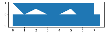
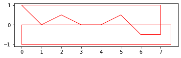
We can use the color and edgecolor parameters to specify the fill color and border color, respectively:

gdf.plot(color="none", edgecolor="red");

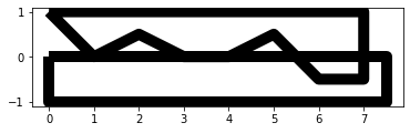
Another useful property is linewidth, to specify line width:

gdf.plot(color='none', linewidth=10);

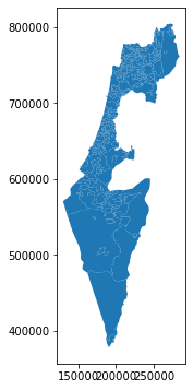
Let us also plot the towns and rail layers to see what they look like:

towns.plot();

rail.plot();

Setting symbology

By default, all plotted geometries share the same appearance. We can set a symbology, where the appearance corresponds to given attributes values, using the column parameter. For example, the following expression results in a map where town fill colors correspond to the "Machoz" attribute values. We can therefore see the “Machoz” administrative division:

towns.plot(column='Machoz');

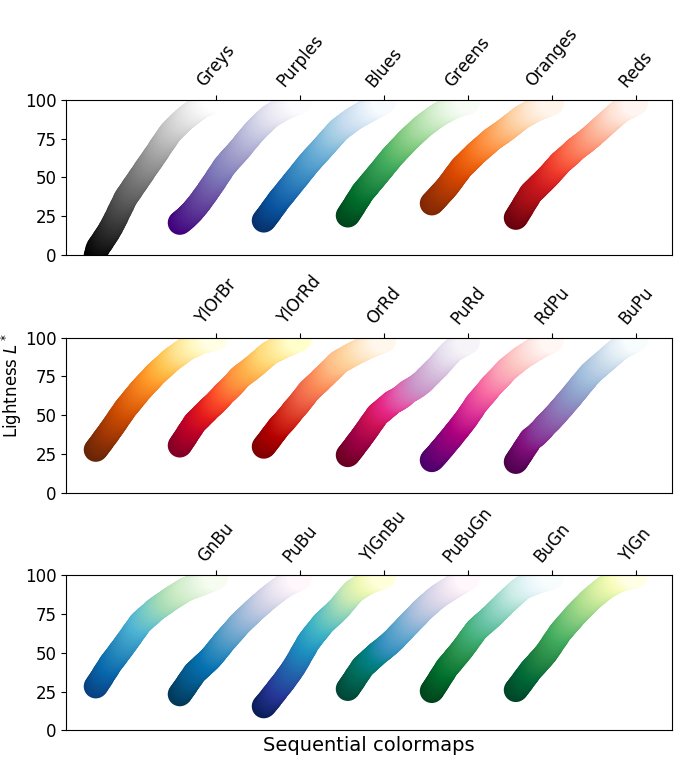
The color palette for the symbology can be changed using the cmap (“color map”) argument. Valid palette names can be found in the Choosing Colormaps page of the matplotlib documentation. For example, "Set2" is one of the “Qualitative colormaps”, which is appropriate for categorical variables:

towns.plot(column='Machoz', cmap='Set2');

As another example, the following expression sets a symbology corresponding to the continuous "Shape_Area" (town area in square meters) columns. The argument legend=True adds a legend:

towns.plot(column='Shape_Area', cmap='Reds', legend=True);

Interactive maps

geopandas also provides the .explore method, which facilitates interactive exploration of the vector layers we are working with. The .explore method takes many of the same arguments as .plot (such as column and cmap), but also some specific ones (such as style_kwds). See the documentation for details.

For example, the following expression creates an interactive map displaying the rail layer, colored according to status (active or not). Note that hovering over a feature with the mouse shows a tooltip with the attribute values (similarly to “identify” tools in GIS software).

rail.explore(column='ISACTIVE', cmap='RdYlBu', style_kwds={'weight':8, 'opacity':0.8})

Make this Notebook Trusted to load map: File -> Trust Notebook

Note

There are several Python packages for creating interactive maps displaying spatial data, either inside a Jupyter notebook or exporting to an HTML document. Most notably, these include folium, ipyleaflet, leafmap, and bokeh. All but the last one are based on the Leaflet web-mapping JavaScript package. The .explore method of geopandas, in fact, uses the folium package and requires it to be installed.

Plotting more than one layer

It is is often helpful to display several layers together in the same plot, one on top of the other. That way, we can see the orientation and alignment of several layers at once.

To display two or more layers in the same geopandas plot, we need to do things a little differently than shown above (see Basic plots):

• First, we need to assign a specific plot (with one of the layers), to a variable, such as base. This serves as the “base” plot.

• Then, we can display any additional layer on top of the base plot using its .plot method, while passing the base plot object to the ax parameter, as in ax=base.

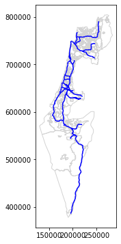
For example, here is how we can plot both towns and rail, one on top of the other. Note that we use color="none" for transparent fill of the polygons:

base = towns.plot(color='none', edgecolor='lightgrey')
rail.plot(ax=base, color='blue');

Note

More information on plotting geopandas layers can be found in https://geopandas.org/docs/user_guide/mapping.html.

Selecting GeoDataFrame columns

We can subset columns in a GeoDataFrame the same way as in a DataFrame, using the [[ operator (see Selecting DataFrame columns). The only thing we need to keep in mind is that we must keep the "geometry" column, so that the result remains a vector layer rather than an ordinary table.

For example, the following expression subsets 5 out of the 23 columns in towns:

towns = towns[["Muni_Heb", "Muni_Eng", "Machoz", "Shape_Area", "geometry"]]
towns

	Muni_Heb	Muni_Eng	Machoz	Shape_Area	geometry
0	ללא שיפוט - אזור מעיליא	No Jurisdiction - Mi'ilya Area	צפון	2.001376e+05	POLYGON Z ((225369.655 770523.6...
1	תמר	Tamar	דרום	1.597418e+09	POLYGON Z ((206899.135 552967.8...
2	שהם	Shoham	מרכז	6.177438e+06	POLYGON Z ((194329.250 655299.1...
3	שהם	Shoham	מרכז	9.850450e+05	POLYGON Z ((196236.573 657835.0...
4	ראש פינה	Rosh Pina	צפון	6.104233e+04	POLYGON Z ((255150.135 764764.6...
...	...	...	...	...	...
405	אופקים	Ofakim	דרום	1.635240e+07	POLYGON Z ((164806.146 577898.8...
406	אבן יהודה	Even Yehuda	מרכז	8.141962e+06	POLYGON Z ((189803.359 684152.9...
407	אבו סנאן	Abu Snan	צפון	6.455340e+06	POLYGON Z ((212294.953 763168.8...
408	אבו גוש	Abu Gosh (Abu Rosh)	ירושלים	1.891242e+06	POLYGON Z ((209066.649 635655.2...
409	שדות נגב	Sdot Negev	דרום	2.554627e+05	POLYGON Z ((162082.027 592043.1...

410 rows × 5 columns

And here we subset three of the columns in rail:

rail = rail[['SEGMENT', 'ISACTIVE', 'geometry']]
rail

	SEGMENT	ISACTIVE	geometry
0	כפר יהושע - נשר_1	פעיל	LINESTRING (205530.083 741562.9...
1	באר יעקב-ראשונים_2	פעיל	LINESTRING (181507.598 650706.1...
2	נתבג - נען_3	לא פעיל	LINESTRING (189180.643 645433.4...
3	לב המפרץ מזרח - נשר_4	פעיל	LINESTRING (203482.789 744181.5...
4	קרית גת - להבים_5	פעיל	LINESTRING (178574.101 609392.9...
...	...	...	...
212	ראש העין צפון - כפר סבא צפון_	לא פעיל	LINESTRING (195887.590 675861.9...
213	רמלה דרום-ראשונים_218	לא פעיל	LINESTRING (183225.361 648648.2...
214	השמונה - בית המכס_220	פעיל	LINESTRING (200874.999 746209.3...
215	לב המפרץ - בית המכס_221	פעיל	LINESTRING (203769.786 744358.6...
216	224_לוד מרכז - נתבג	פעיל	LINESTRING (190553.481 654170.3...

217 rows × 3 columns

Filtering by attributes

We can subset the rows (i.e., features) of a GeoDataFrame using a corresponding boolean Series, the same way we subset rows of a DataFrame (see DataFrame filtering). Typically, the boolean Series is the result of applying a conditional operator on one or more columns of the same GeoDataFrame.

For example, suppose that we want to retain just the active railway segments from the rail layer, namely those segments where the value in the "ISACTIVE" column is equal to "פעיל" (“active”). First, we need to create a boolean series where True values reflect the rows we would like to retain. Here, we assign the boolean Series to a variable named sel:

sel = rail['ISACTIVE'] == 'פעיל'
sel

0       True
1       True
2      False
3       True
4       True
       ...  
212    False
213    False
214     True
215     True
216     True
Name: ISACTIVE, Length: 217, dtype: bool

Second, we need to pass the series as an index to the GeoDataFrame. As a result, rail now contains only the active railway lines (161 features out of 217):

rail = rail[sel]
rail

	SEGMENT	ISACTIVE	geometry
0	כפר יהושע - נשר_1	פעיל	LINESTRING (205530.083 741562.9...
1	באר יעקב-ראשונים_2	פעיל	LINESTRING (181507.598 650706.1...
3	לב המפרץ מזרח - נשר_4	פעיל	LINESTRING (203482.789 744181.5...
4	קרית גת - להבים_5	פעיל	LINESTRING (178574.101 609392.9...
5	רמלה - רמלה מזרח_6	פעיל	LINESTRING (189266.580 647211.5...
...	...	...	...
210	ויתקין - חדרה_215	פעיל	LINESTRING (190758.230 704950.0...
211	בית יהושע - נתניה ספיר_216	פעיל	LINESTRING (187526.597 687360.3...
214	השמונה - בית המכס_220	פעיל	LINESTRING (200874.999 746209.3...
215	לב המפרץ - בית המכס_221	פעיל	LINESTRING (203769.786 744358.6...
216	224_לוד מרכז - נתבג	פעיל	LINESTRING (190553.481 654170.3...

161 rows × 3 columns

Once you are more comfortable with the subsetting syntax you may prefer to do the operation in a single step, as follows:

rail = rail[rail['ISACTIVE'] == 'פעיל']

Let us plot the filtered rail layer, to see the effect visually:

rail.plot();

Exercise 08-a

• The layer statisticalareas_demography2019.gdb contains demographic data for the statistical areas of Israel, such as population size per age group, in 2019. For example, the column "age_10_14" contains population counts in the 10-14 age group, while the "Pop_Total" column contains total population counts (in all age groups). Note that statisticalareas_demography2019.gdb is in a format known as a File Geodatabase.

• Read the statisticalareas_demography2019.gdb layer into a GeoDataFrame.

• Subset the following columns (plus the geometry!):

  • "YISHUV_STAT11"—Statistical area ID

  • "SHEM_YISHUV"—Town name in Hebrew

  • "SHEM_YISHUV_ENGLISH"—Town name in English

  • "Pop_Total"—Total population size

• What is the Coordinate Reference System of the layer? (answer: "Israel 1993 / Israeli TM Grid", i.e., “ITM”)

• How many features does the layer contain? Write an expression that returns the result as int. (answer: 3195)

• The values in the "YISHUV_STAT11" column (statistical area ID) should all be unique. How can you make sure? Either use one of the methods we learned earlier, or search online (e.g., google “pandas check for duplicates”).

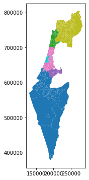
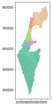
• Plot the layer using the .plot method (Fig. 48).

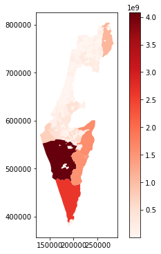
• Subset just the statistical areas of Beer-Sheva, using either the "SHEM_YISHUV" or the "SHEM_YISHUV_ENGLISH" column.

• Plot the resulting subset, using symbology according to total population size, i.e., the "Pop_Total" column, and using a sequentual color map such as "Reds" (Fig. 49).

• How many statistical areas are there in Beer-Sheva? (answer: 62)

• What was the total population of Beer-Sheva in 2019? (answer: 209685.0)

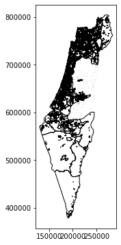
Fig. 48 Solution of exercise-08-a1: The statistical areas layer

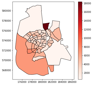
Fig. 49 Solution of exercise-08-a2: Statistical areas of Beer-Sheva, with symbology according to total population size

Table to point layer

Another very common workflow of creating a vector layer is creating a point layer from a table that has X and Y coordinates in two separate columns. Technically, this means that the X and Y values in each row are transformed into a "Point" geometry. The geometries are then placed in a geometry column, so that the table becomes a vector layer.

To demonstrate, let us import the stops.txt table, which contains information about public transport stops in Israel based on GTFS data (see What is GTFS?). Note the columns stop_lon and stop_lat, which contain the X and Y coordinates, in the WGS84 coordinate system, i.e., longitude and latitude, respectively:

stops = pd.read_csv('data/gtfs/stops.txt')
stops = stops[['stop_id', 'stop_name', 'stop_lon', 'stop_lat']]
stops

	stop_id	stop_name	stop_lon	stop_lat
0	1	בי''ס בר לב/בן יהודה	34.917554	32.183985
1	2	הרצל/צומת בילו	34.819541	31.870034
2	3	הנחשול/הדייגים	34.782828	31.984553
3	6	ת. מרכזית לוד/הורדה	34.898098	31.956392
4	8	הרצל/משה שרת	34.824106	31.857565
...	...	...	...	...
28250	44668	חניון שפירים דרומי/הורדה	34.840406	32.001228
28251	44683	מתחם נצבא	34.941549	32.112445
28252	44684	מתחם נצבא	34.940668	32.111795
28253	44691	מסוף דרך שכם	35.228825	31.783680
28254	44692	הקוממיות/אנה פרנק	34.752376	32.002782

28255 rows × 4 columns

To transform a DataFrame with X and Y columns into a GeoDataFrame point layer, we go through two steps:

• Constructing a GeoSeries of "Point" geometries, from two Series representing X and Y, using gpd.points_from_xy. Optionally, we can specify the CRS of the GeoSeries, using the crs parameter.

• Converting the GeoSeries to a GeoDataFrame, using gpd.GeoDataFrame.

Let us begin with the first step—creating the GeoSeries. The X and Y columns are readily available, stops["stop_lon"], stops["stop_lat"], however specifying the crs parameter is less trivial. The CRS definition is usually not stored in the same table with the X and Y columns, since it would have to be repeated on all rows. We need to figure out which CRS the X and Y coordinates are in according to the metadata or accompanying information (such as the GTFS specification). In this particular case, the names stop_lon and stop_lat (where lon=longitude and lat=latitude) give a pretty good hint that the coordinates are given in WGS84, therefore we use crs=4326:

geom = gpd.points_from_xy(stops['stop_lon'], stops['stop_lat'], crs=4326)

The result is a special type of array named GeometryArray:

type(geom)

geopandas.array.GeometryArray

Though it can be used as is, we are going to convert it to a GeoSeries, which we are already familiar with, for clarity:

geom = gpd.GeoSeries(geom)
geom

0        POINT (34.91755 32.18398)
1        POINT (34.81954 31.87003)
2        POINT (34.78283 31.98455)
3        POINT (34.89810 31.95639)
4        POINT (34.82411 31.85757)
                   ...            
28250    POINT (34.84041 32.00123)
28251    POINT (34.94155 32.11245)
28252    POINT (34.94067 32.11180)
28253    POINT (35.22883 31.78368)
28254    POINT (34.75238 32.00278)
Length: 28255, dtype: geometry

Now, we can use the gpd.GeoDataFrame function to combine the DataFrame with the GeoSeries, to get a GeoDataFrame. Instead of passing a dict of columns, like we did when creating a layer manually (see Creating a GeoDataFrame), we pass a DataFrame and a GeoSeries to the data and geometry parameters, respectively:

stops = gpd.GeoDataFrame(data=stops, geometry=geom)
stops

	stop_id	stop_name	stop_lon	stop_lat	geometry
0	1	בי''ס בר לב/בן יהודה	34.917554	32.183985	POINT (34.91755 32.18398)
1	2	הרצל/צומת בילו	34.819541	31.870034	POINT (34.81954 31.87003)
2	3	הנחשול/הדייגים	34.782828	31.984553	POINT (34.78283 31.98455)
3	6	ת. מרכזית לוד/הורדה	34.898098	31.956392	POINT (34.89810 31.95639)
4	8	הרצל/משה שרת	34.824106	31.857565	POINT (34.82411 31.85757)
...	...	...	...	...	...
28250	44668	חניון שפירים דרומי/הורדה	34.840406	32.001228	POINT (34.84041 32.00123)
28251	44683	מתחם נצבא	34.941549	32.112445	POINT (34.94155 32.11245)
28252	44684	מתחם נצבא	34.940668	32.111795	POINT (34.94067 32.11180)
28253	44691	מסוף דרך שכם	35.228825	31.783680	POINT (35.22883 31.78368)
28254	44692	הקוממיות/אנה פרנק	34.752376	32.002782	POINT (34.75238 32.00278)

28255 rows × 5 columns

The "stop_lon" and "stop_lat" columns are no longer necessary, because the information is already in the "geometry" columns. Therefore, they can be dropped:

stops = stops.drop(['stop_lon', 'stop_lat'], axis=1)
stops

	stop_id	stop_name	geometry
0	1	בי''ס בר לב/בן יהודה	POINT (34.91755 32.18398)
1	2	הרצל/צומת בילו	POINT (34.81954 31.87003)
2	3	הנחשול/הדייגים	POINT (34.78283 31.98455)
3	6	ת. מרכזית לוד/הורדה	POINT (34.89810 31.95639)
4	8	הרצל/משה שרת	POINT (34.82411 31.85757)
...	...	...	...
28250	44668	חניון שפירים דרומי/הורדה	POINT (34.84041 32.00123)
28251	44683	מתחם נצבא	POINT (34.94155 32.11245)
28252	44684	מתחם נצבא	POINT (34.94067 32.11180)
28253	44691	מסוף דרך שכם	POINT (35.22883 31.78368)
28254	44692	הקוממיות/אנה פרנק	POINT (34.75238 32.00278)

28255 rows × 3 columns

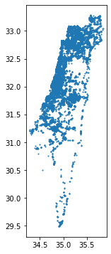
Plotting the resulting layer of public transport stations reveals the outline of Israel, with more sparse coverage in the southern part, which corresponds to population density pattern in the country. The markersize argument is used to for smaller point size to reduce overlap:

stops.plot(markersize=1);

Points to line (geopandas)

To lines: all points combined

A common type of geometry casting, which we already met when learning about shapely is the transformation of points to lines (see Points to line (shapely)). Let us see how this type of casting can be acheived when our points are in a GeoDataFrame. We begin, in this section, with transforming an entire point layer to a single continuous line. In the next section, we will learn how to transform a point layer to a layer with multiple lines by group (see To lines: by group).

To demonstrate, let us import the shapes.txt table (see What is GTFS?) from the GTFS dataset. This table contains the shapes of public transit lines. This is quite a big table, with over 7 million rows. In the table, each shape is distinguished by a unique "shape_id", comprised of lon/lat coordinates in the "shape_pt_lat", "shape_pt_lon" columns:

shapes = pd.read_csv('data/gtfs/shapes.txt')
shapes

	shape_id	shape_pt_lat	shape_pt_lon	shape_pt_sequence
0	44779	31.887695	35.016271	1
1	44779	31.887745	35.016253	2
2	44779	31.888256	35.016238	3
3	44779	31.888913	35.016280	4
4	44779	31.888917	35.016892	5
...	...	...	...	...
7226268	123167	32.729572	35.331201	876
7226269	123167	32.729700	35.330923	877
7226270	123167	32.729706	35.330908	878
7226271	123167	32.729841	35.330538	879
7226272	123167	32.729899	35.330249	880

7226273 rows × 4 columns

For the first example, we take a subset of shapes containing the shape of just one transit line. We will select the 118789 value of "shape_id", which corresponds to bus line 24 in Beer-Sheva going from Ramot to Beer-Sheva Central Bus Station (see Solution of exercise-07-i: bus stops as points). This results in a much smaller table, with 828 rows:

pnt = shapes[shapes["shape_id"] == 118789]
pnt

	shape_id	shape_pt_lat	shape_pt_lon	shape_pt_sequence
4264621	118789	31.280061	34.821551	1
4264622	118789	31.280038	34.821704	2
4264623	118789	31.280023	34.821880	3
4264624	118789	31.280022	34.822029	4
4264625	118789	31.280031	34.822072	5
...	...	...	...	...
4265444	118789	31.242103	34.797988	826
4265445	118789	31.242829	34.797982	827
4265446	118789	31.242980	34.797986	828
4265447	118789	31.243121	34.798000	829
4265448	118789	31.243263	34.798017	830

828 rows × 4 columns

What we have is a DataFrame with x/y coordinate columns, "shape_pt_lon" and "shape_pt_lat". We already know how to transform it to a GeoDataFrame with point geometries (see Table to point layer):

geom = gpd.points_from_xy(pnt['shape_pt_lon'], pnt['shape_pt_lat'], crs=4326)
pnt = gpd.GeoDataFrame(data=pnt, geometry=geom)
pnt

	shape_id	shape_pt_lat	shape_pt_lon	shape_pt_sequence	geometry
4264621	118789	31.280061	34.821551	1	POINT (34.82155 31.28006)
4264622	118789	31.280038	34.821704	2	POINT (34.82170 31.28004)
4264623	118789	31.280023	34.821880	3	POINT (34.82188 31.28002)
4264624	118789	31.280022	34.822029	4	POINT (34.82203 31.28002)
4264625	118789	31.280031	34.822072	5	POINT (34.82207 31.28003)
...	...	...	...	...	...
4265444	118789	31.242103	34.797988	826	POINT (34.79799 31.24210)
4265445	118789	31.242829	34.797982	827	POINT (34.79798 31.24283)
4265446	118789	31.242980	34.797986	828	POINT (34.79799 31.24298)
4265447	118789	31.243121	34.798000	829	POINT (34.79800 31.24312)
4265448	118789	31.243263	34.798017	830	POINT (34.79802 31.24326)

828 rows × 5 columns

The "shape_pt_lat" and "shape_pt_lon" columns are no longer necessary and can be dropped:

pnt = pnt.drop(['shape_pt_lon', 'shape_pt_lat'], axis=1)
pnt

	shape_id	shape_pt_sequence	geometry
4264621	118789	1	POINT (34.82155 31.28006)
4264622	118789	2	POINT (34.82170 31.28004)
4264623	118789	3	POINT (34.82188 31.28002)
4264624	118789	4	POINT (34.82203 31.28002)
4264625	118789	5	POINT (34.82207 31.28003)
...	...	...	...
4265444	118789	826	POINT (34.79799 31.24210)
4265445	118789	827	POINT (34.79798 31.24283)
4265446	118789	828	POINT (34.79799 31.24298)
4265447	118789	829	POINT (34.79800 31.24312)
4265448	118789	830	POINT (34.79802 31.24326)

828 rows × 3 columns

Now, we are going use shapely to transform the point geometries into a single "LineString" geometry. First, we create a list of shapely geometries, which requires selecting the GeoSeries (geometry) column and converting it to a list the using .to_list method (see Individual geometries):

x = pnt['geometry'].to_list()
x[:5]

[<shapely.geometry.point.Point at 0x7f4c1dfacb80>,
 <shapely.geometry.point.Point at 0x7f4c1ff23bb0>,
 <shapely.geometry.point.Point at 0x7f4c1fe77010>,
 <shapely.geometry.point.Point at 0x7f4c22ef3a30>,
 <shapely.geometry.point.Point at 0x7f4c1dfafb50>]

Then, we use the shapely.geometry.LineString function (see Points to line (shapely)) to convert the list of "Point" geometries to a single "LineString" geometry, as follows:

line = shapely.geometry.LineString(x)
line

In case we need the geometry to be contained in a GeoDataFrame, rather than a standalone shapely geometry, we can construct a GeoDataFrame using the methods we learned in the beginning of this chapter (see Creating a GeoDataFrame):

line1 = gpd.GeoDataFrame({'geometry': [line]}, crs=4326)
line1

	geometry
0	LINESTRING (34.82155 31.28006, ...

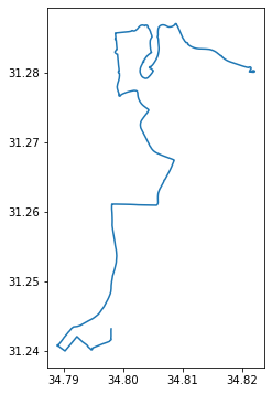
Here is a plot of the resulting layer line1:

line1.plot();

To lines: by group

In the next example, we demonstrate how the conversion of points to lines can be generalized to produce multiple lines at once, in case when there is a grouping variable specifying the division of points to groups. For example, using the GTFS data, we may want to create a layer of type "LineString", with all different bus routes together, rahter than just one specific route (see To lines: all points combined). This example is relatively complex, with many steps to get the data into the right shape.

Our first step is to read four tables from the GTFS dataset, namely agency, routes, trips, and shapes:

agency = pd.read_csv('data/gtfs/agency.txt')
routes = pd.read_csv('data/gtfs/routes.txt')
trips = pd.read_csv('data/gtfs/trips.txt')
shapes = pd.read_csv('data/gtfs/shapes.txt')

We will also subset the most relevant columns of each table, for our purposes:

agency = agency[['agency_id', 'agency_name']]
routes = routes[['route_id', 'agency_id', 'route_short_name', 'route_long_name']]
trips = trips[['trip_id', 'route_id', 'shape_id']]
shapes = shapes[['shape_id', 'shape_pt_sequence', 'shape_pt_lon', 'shape_pt_lat']]

To have a more manageable layer size, we will subset just one bus operator, namely "מטרופולין". First, we need to figure out its agency_id:

agency = agency[agency['agency_name'] == 'מטרופולין']
agency

	agency_id	agency_name
9	15	מטרופולין

Now that we know the agency_id of "מטרופולין", we can subset the routes table to retain only the routes by this particular operator. We also drop the "agency_id" column which is no longer necessary. We can see there are 625 routes operated by "מטרופולין":

routes = routes[routes['agency_id'] == agency['agency_id'].iloc[0]]
routes = routes.drop('agency_id', axis=1)
routes

	route_id	route_short_name	route_long_name
235	696	600	ת. מרכזית נתניה/רציפים-נתניה<->...
236	697	600	ת.מרכזית ת''א ק.6/רציפים-תל אבי...
237	698	601	ת. רכבת נתניה-נתניה<->ת. מרכזית...
238	700	601	ת.מרכזית ת''א ק.6/רציפים-תל אבי...
239	707	604	ת. מרכזית נתניה/רציפים-נתניה<->...
...	...	...	...
7148	28601	80	יהודה/חברון-ערד<->פלמ''ח/עין הת...
7149	28602	64	בי''ס שדה הר הנגב-מצפה רמון<->ת...
7156	28694	561	ת. רכבת קרית אריה-פתח תקווה<->ת...
7200	29130	1	מסוף קדמה-רמת השרון<->מסוף קדמה...
7201	29131	32	בית ברל/מרכז-בית ברל<->מסוף קדמ...

625 rows × 3 columns

Next, we need to join the routes table with the shapes table, where the route coordinates are. However the routes table corresponds to the shapes table indirectly, through the trips table (Fig. 30). Therefore we first need to join trips to routes, and then shapes to the result. To make things simpler, we will remove duplicates from the trips table, assuming that all trips of a particular route follow the same shape (which they typically do), thus retaining just one representative trip per route. Here is the current state of the trips table, with numerous trips per route:

trips

	trip_id	route_id	shape_id
0	28876224_180421	1	121757.0
1	28876225_180421	1	121757.0
2	28876226_180421	1	121757.0
3	28876227_180421	1	121757.0
4	28876228_180421	1	121757.0
...	...	...	...
287673	56622686_230421	29363	123144.0
287674	56460152_180421	29364	NaN
287675	56458677_180421	29365	67648.0
287676	56458667_180421	29366	51396.0
287677	56458657_180421	29368	123033.0

287678 rows × 3 columns

To remove duplicates from a table, we can use the .drop_duplicates method. This method accepts an argument named subset, where we specify which column(s) are considered for duplicates. In our case, we remove rows with duplicated route_id in trips, thus retaining just one route_id per trip:

trips = trips.drop_duplicates(subset='route_id')
trips

	trip_id	route_id	shape_id
0	28876224_180421	1	121757.0
45	25448344_180421	2	121758.0
88	56334623_180421	3	97106.0
119	56335137_180421	5	121759.0
154	37173391_180421	7	119801.0
...	...	...	...
287668	56622661_230421	29363	123144.0
287674	56460152_180421	29364	NaN
287675	56458677_180421	29365	67648.0
287676	56458667_180421	29366	51396.0
287677	56458657_180421	29368	123033.0

7251 rows × 3 columns

We can also drop the trip_id column, which is no longer necessary:

trips = trips.drop('trip_id', axis=1)
trips

	route_id	shape_id
0	1	121757.0
45	2	121758.0
88	3	97106.0
119	5	121759.0
154	7	119801.0
...	...	...
287668	29363	123144.0
287674	29364	NaN
287675	29365	67648.0
287676	29366	51396.0
287677	29368	123033.0

7251 rows × 2 columns

Now we can run both joins:

• first joining trips to routes, to attach the shape IDs,

• then shapes to the result, to attach the lon/lat point sequences

as follows:

routes

	route_id	route_short_name	route_long_name
235	696	600	ת. מרכזית נתניה/רציפים-נתניה<->...
236	697	600	ת.מרכזית ת''א ק.6/רציפים-תל אבי...
237	698	601	ת. רכבת נתניה-נתניה<->ת. מרכזית...
238	700	601	ת.מרכזית ת''א ק.6/רציפים-תל אבי...
239	707	604	ת. מרכזית נתניה/רציפים-נתניה<->...
...	...	...	...
7148	28601	80	יהודה/חברון-ערד<->פלמ''ח/עין הת...
7149	28602	64	בי''ס שדה הר הנגב-מצפה רמון<->ת...
7156	28694	561	ת. רכבת קרית אריה-פתח תקווה<->ת...
7200	29130	1	מסוף קדמה-רמת השרון<->מסוף קדמה...
7201	29131	32	בית ברל/מרכז-בית ברל<->מסוף קדמ...

625 rows × 3 columns

routes = pd.merge(routes, trips, on='route_id', how='left')
routes

	route_id	route_short_name	route_long_name	shape_id
0	696	600	ת. מרכזית נתניה/רציפים-נתניה<->...	120512.0
1	697	600	ת.מרכזית ת''א ק.6/רציפים-תל אבי...	119606.0
2	698	601	ת. רכבת נתניה-נתניה<->ת. מרכזית...	112496.0
3	700	601	ת.מרכזית ת''א ק.6/רציפים-תל אבי...	120629.0
4	707	604	ת. מרכזית נתניה/רציפים-נתניה<->...	120513.0
...	...	...	...	...
620	28601	80	יהודה/חברון-ערד<->פלמ''ח/עין הת...	120656.0
621	28602	64	בי''ס שדה הר הנגב-מצפה רמון<->ת...	120663.0
622	28694	561	ת. רכבת קרית אריה-פתח תקווה<->ת...	120954.0
623	29130	1	מסוף קדמה-רמת השרון<->מסוף קדמה...	122862.0
624	29131	32	בית ברל/מרכז-בית ברל<->מסוף קדמ...	122381.0

625 rows × 4 columns

routes = pd.merge(routes, shapes, on='shape_id', how='left')
routes

	route_id	route_short_name	route_long_name	...	shape_pt_sequence	shape_pt_lon	shape_pt_lat
0	696	600	ת. מרכזית נתניה/רציפים-נתניה<->...	...	1	34.858567	32.326985
1	696	600	ת. מרכזית נתניה/רציפים-נתניה<->...	...	2	34.859270	32.326788
2	696	600	ת. מרכזית נתניה/רציפים-נתניה<->...	...	3	34.859413	32.326743
3	696	600	ת. מרכזית נתניה/רציפים-נתניה<->...	...	4	34.859245	32.326359
4	696	600	ת. מרכזית נתניה/רציפים-נתניה<->...	...	5	34.858540	32.326587
...	...	...	...	...	...	...	...
541593	29131	32	בית ברל/מרכז-בית ברל<->מסוף קדמ...	...	916	34.860352	32.129688
541594	29131	32	בית ברל/מרכז-בית ברל<->מסוף קדמ...	...	917	34.860269	32.129663
541595	29131	32	בית ברל/מרכז-בית ברל<->מסוף קדמ...	...	918	34.860215	32.129636
541596	29131	32	בית ברל/מרכז-בית ברל<->מסוף קדמ...	...	919	34.860143	32.129589
541597	29131	32	בית ברל/מרכז-בית ברל<->מסוף קדמ...	...	920	34.860047	32.129520

541598 rows × 7 columns

The resulting routes table contains, in the shape_pt_lon and shape_pt_lat, the coordinate sequence per route_id. Now, we can move on to the spatial part of the conversion, where the table will be transformed to a "LineString" layer of routes.

First, we convert the DataFrame to a GeoDataFrame of type "Point", same as we did above for the individual line number 24 in Beer-Sheva (see To lines: all points combined):

geom = gpd.points_from_xy(routes['shape_pt_lon'], routes['shape_pt_lat'], crs=4326)
routes = gpd.GeoDataFrame(data=routes, geometry=geom)
routes = routes.drop(['shape_pt_lon', 'shape_pt_lat'], axis=1)
routes

	route_id	route_short_name	route_long_name	shape_id	shape_pt_sequence	geometry
0	696	600	ת. מרכזית נתניה/רציפים-נתניה<->...	120512.0	1	POINT (34.85857 32.32699)
1	696	600	ת. מרכזית נתניה/רציפים-נתניה<->...	120512.0	2	POINT (34.85927 32.32679)
2	696	600	ת. מרכזית נתניה/רציפים-נתניה<->...	120512.0	3	POINT (34.85941 32.32674)
3	696	600	ת. מרכזית נתניה/רציפים-נתניה<->...	120512.0	4	POINT (34.85925 32.32636)
4	696	600	ת. מרכזית נתניה/רציפים-נתניה<->...	120512.0	5	POINT (34.85854 32.32659)
...	...	...	...	...	...	...
541593	29131	32	בית ברל/מרכז-בית ברל<->מסוף קדמ...	122381.0	916	POINT (34.86035 32.12969)
541594	29131	32	בית ברל/מרכז-בית ברל<->מסוף קדמ...	122381.0	917	POINT (34.86027 32.12966)
541595	29131	32	בית ברל/מרכז-בית ברל<->מסוף קדמ...	122381.0	918	POINT (34.86021 32.12964)
541596	29131	32	בית ברל/מרכז-בית ברל<->מסוף קדמ...	122381.0	919	POINT (34.86014 32.12959)
541597	29131	32	בית ברל/מרכז-בית ברל<->מסוף קדמ...	122381.0	920	POINT (34.86005 32.12952)

541598 rows × 6 columns

If we needed to convert all sequences into a single "LineString", we could use the method shown earlier (see To lines: all points combined). However, what we need is to create a separate "LineString" per "route_id". Therefore, we:

• Group the layer by "shape_id", using the .agg method (see Different functions (agg))

• Use the "first" “function” to keep the first "route_short_name" and "route_long_name" values per route (as they identical for each "route_id" anyway)

• Apply a lambda function (see Custom functions (agg)) that “summarizes” the "Point" geometries into a "LineString" geometry

Here is the code:

routes = routes.groupby('route_id').agg({
    'route_short_name': 'first',
    'route_long_name': 'first',
    'geometry': lambda x: shapely.geometry.LineString(x.to_list()),
}).reset_index()
routes

	route_id	route_short_name	route_long_name	geometry
0	696	600	ת. מרכזית נתניה/רציפים-נתניה<->...	LINESTRING (34.85857 32.32699, ...
1	697	600	ת.מרכזית ת''א ק.6/רציפים-תל אבי...	LINESTRING (34.77978 32.05568, ...
2	698	601	ת. רכבת נתניה-נתניה<->ת. מרכזית...	LINESTRING (34.86805 32.31966, ...
3	700	601	ת.מרכזית ת''א ק.6/רציפים-תל אבי...	LINESTRING (34.77978 32.05568, ...
4	707	604	ת. מרכזית נתניה/רציפים-נתניה<->...	LINESTRING (34.85857 32.32699, ...
...	...	...	...	...
620	28601	80	יהודה/חברון-ערד<->פלמ''ח/עין הת...	LINESTRING (35.20976 31.25571, ...
621	28602	64	בי''ס שדה הר הנגב-מצפה רמון<->ת...	LINESTRING (34.79048 30.60273, ...
622	28694	561	ת. רכבת קרית אריה-פתח תקווה<->ת...	LINESTRING (34.86472 32.10658, ...
623	29130	1	מסוף קדמה-רמת השרון<->מסוף קדמה...	LINESTRING (34.86035 32.12969, ...
624	29131	32	בית ברל/מרכז-בית ברל<->מסוף קדמ...	LINESTRING (34.92596 32.20191, ...

625 rows × 4 columns

The .groupby and .agg workflow unfortunately “loses” the spatial properties of the data structure, going back to a DataFrame:

type(routes)

pandas.core.frame.DataFrame

Therefore, we need to convert the result back to a GeoDataFrame and restore the CRS information which was lost, using gpd.GeoDataFrame:

routes = gpd.GeoDataFrame(routes, crs=4326)
routes

	route_id	route_short_name	route_long_name	geometry
0	696	600	ת. מרכזית נתניה/רציפים-נתניה<->...	LINESTRING (34.85857 32.32699, ...
1	697	600	ת.מרכזית ת''א ק.6/רציפים-תל אבי...	LINESTRING (34.77978 32.05568, ...
2	698	601	ת. רכבת נתניה-נתניה<->ת. מרכזית...	LINESTRING (34.86805 32.31966, ...
3	700	601	ת.מרכזית ת''א ק.6/רציפים-תל אבי...	LINESTRING (34.77978 32.05568, ...
4	707	604	ת. מרכזית נתניה/רציפים-נתניה<->...	LINESTRING (34.85857 32.32699, ...
...	...	...	...	...
620	28601	80	יהודה/חברון-ערד<->פלמ''ח/עין הת...	LINESTRING (35.20976 31.25571, ...
621	28602	64	בי''ס שדה הר הנגב-מצפה רמון<->ת...	LINESTRING (34.79048 30.60273, ...
622	28694	561	ת. רכבת קרית אריה-פתח תקווה<->ת...	LINESTRING (34.86472 32.10658, ...
623	29130	1	מסוף קדמה-רמת השרון<->מסוף קדמה...	LINESTRING (34.86035 32.12969, ...
624	29131	32	בית ברל/מרכז-בית ברל<->מסוף קדמ...	LINESTRING (34.92596 32.20191, ...

625 rows × 4 columns

type(routes)

geopandas.geodataframe.GeoDataFrame

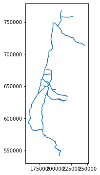
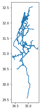
Here is a plot of the result. This is a line layer of all 625 routes operated by the "מטרופולין" agency, reflecting the shape of the first representative trip per route:

routes.plot();

Exercise 08-b

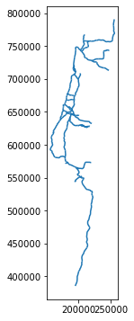
• Repeat creation of the line layer routes, as shown above, but this time subset the operator "דן באר שבע".

• Calcualte a GeoSeries of starting points of each route. Hint: you can either go over the "LineString" geometries and extract the first point using shapely methods (see LineString coordinates and shapely from type-specific functions), or go back to the point layer and subset the first point per route_id.

• Plot the routes and the start points together (Fig. 50).

• Note that the default plotting order of matplotlib is lines on top of points. To have points on top of lines, specify:

  • zorder=1 when plotting the lines, and

  • zorder=2 when plotting the points.

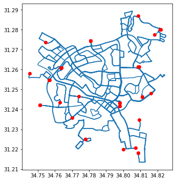
Fig. 50 Solution of exercise-08-b: Routes operated by "דן באר שבע" and their start points

We can also explore the routes, or some of them, interactively (see Interactive maps). For example, the following expression displays bus lines "367", "368", and "370", which travel between Beer-Sheva, and Rishon Le Zion ("367"), Ashdod ("368"), and Tel-Aviv ("370"). Note that we are using the .isin method (see Using .isin) for filtering:

routes1 = routes[routes['route_short_name'].isin(['367', '368', '370'])]
routes1

	route_id	route_short_name	route_long_name	geometry
194	8140	367	ת. מרכזית רשל''צ/רציפים-ראשון ל...	LINESTRING (34.78518 31.96795, ...
195	8141	367	ת.מרכזית באר שבע/רציפים בינעירו...	LINESTRING (34.79679 31.24297, ...
196	8145	368	ת. מרכזית אשדוד/רציפים-אשדוד<->...	LINESTRING (34.63879 31.79072, ...
197	8148	368	ת.מרכזית באר שבע/רציפים בינעירו...	LINESTRING (34.79679 31.24297, ...
204	8170	370	ת.מרכזית ת''א ק.6/רציפים-תל אבי...	LINESTRING (34.77978 32.05568, ...
205	8171	370	ת.מרכזית באר שבע/רציפים בינעירו...	LINESTRING (34.79679 31.24297, ...

Typically, there are two routes for each line, one route per direction, labelled 1# and 2#, which is why we got six routes for three lines:

routes1['route_long_name'].to_list()

["ת. מרכזית רשל''צ/רציפים-ראשון לציון<->ת.מרכזית באר שבע/הורדה-באר שבע-1#",
 "ת.מרכזית באר שבע/רציפים בינעירוני-באר שבע<->ת. מרכזית ראשל''צ-ראשון לציון-2#",
 'ת. מרכזית אשדוד/רציפים-אשדוד<->ת.מרכזית באר שבע/הורדה-באר שבע-1#',
 'ת.מרכזית באר שבע/רציפים בינעירוני-באר שבע<->ת. מרכזית אשדוד-אשדוד-2#',
 "ת.מרכזית ת''א ק.6/רציפים-תל אביב יפו<->ת.מרכזית באר שבע/הורדה-באר שבע-1#",
 "ת.מרכזית באר שבע/רציפים בינעירוני-באר שבע<->ת. מרכזית ת''א ק. 6/הורדה-תל אביב יפו-2#"]

When mapping the lines we can keep just one, since the routes of the same line in both directions mostly overlap anyway:

routes1 = routes1.drop_duplicates('route_short_name')
routes1

	route_id	route_short_name	route_long_name	geometry
194	8140	367	ת. מרכזית רשל''צ/רציפים-ראשון ל...	LINESTRING (34.78518 31.96795, ...
196	8145	368	ת. מרכזית אשדוד/רציפים-אשדוד<->...	LINESTRING (34.63879 31.79072, ...
204	8170	370	ת.מרכזית ת''א ק.6/רציפים-תל אבי...	LINESTRING (34.77978 32.05568, ...

Here is an interactive map of the three lines. Here we use another option for specifying cmap, using specific color names (which is specific to .explore):

routes1.explore(column='route_short_name', cmap=['red', 'green', 'blue'], style_kwds={'weight':8, 'opacity':0.8})

Make this Notebook Trusted to load map: File -> Trust Notebook

Writing vector layers

A GeoDataFrame can be written to file using its .to_file method. This is useful for:

• Permanent storage of the data, for future analysis or for sharing your results with other people

• Examining the result in other software, such as GIS software, for validation or exploration of your results

The default output format of .to_file is the Shapefile. For example, the following expression writes the routes line layer (see To lines: by group) into a Shapefile named routes.shp in the output directory. When exporting a Shapefile with non-English text, we sould also specify the encoding, such as encoding="utf-8":

routes.to_file('output/routes.shp', encoding='utf-8')

/tmp/ipykernel_13058/666508242.py:1: UserWarning: Column names longer than 10 characters will be truncated when saved to ESRI Shapefile.
  routes.to_file('output/routes.shp', encoding='utf-8')

Now we can permanently store the layer of bus routes, share it with a colleague, or open it in another program such as QGIS (Fig. 51).

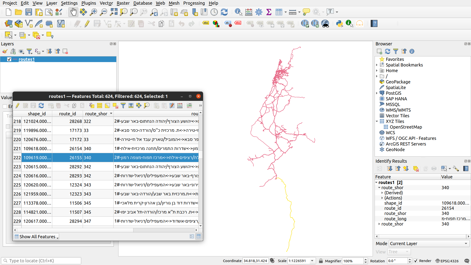
Fig. 51 The routes layer, exported to Shapefile and opened in QGIS

Writing to GeoJSON and GeoPackage formats is similar, only that we need to specify the driver name using the string "GeoJSON" or "GPKG", respectively:

routes.to_file('output/routes.geojson', driver='GeoJSON')
routes.to_file('output/routes.gpkg', driver='GPKG')

Note that if the output file already exists—it will be overwritten!

More exercises

Exercise 08-c

• In this exercise, you need to use the statistical areas layer (statisticalareas_demography2019.gdb) to find out which towns have the highest, or lowest, proportions of young (0-19) residents. To do that, go through the following steps.

• Read the statistical areas layer (statisticalareas_demography2019.gdb).

• Subset the columns "SHEM_YISHUV", "age_0_4", "age_5_9", "age_10_14", "age_15_19", and "Pop_Total". Note that the result is a DataFrame, since the geometry column was not included.

• Replace the “No Data” values in the "age_0_4", "age_5_9", "age_10_14", "age_15_19", and "Pop_Total" columns with zero (as these represent zero population).

• Sum the "age_0_4", "age_5_9", "age_10_14", and "age_15_19" columns to calculate a new column named "Pop_Total_0_19", which represents the total population in ages 0-19 per polygon.

• Subset only those towns with "Pop_Total" greater than 5000.

• Aggregate by town name ("SHEM_YISHUV" column), while calculating the sum of the "Pop_Total_0_19" and the "Pop_Total" columns.

• Calculate the ratio between the young and total population, by dividing the "Pop_Total_0_19" column by the "Pop_Total" column, and store it in a new column named "ratio".

• Reclassify the "ratio" values into two categories:

  • "young"—Where the "ratio" is above the average of the entire "ratio" column.

  • "old"—Where the "ratio" is below the average of the entire "ratio" column.

• Print the five towns with the highest and lowest "ratio" values (Fig. 52).

	SHEM_YISHUV	age_0_4	age_5_9	age_10_14	age_15_19	Pop_Total	Pop_Total_0_19	ratio	type
149	קריית ביאליק	696.0	646.0	634.0	635.0	10980.0	2611.0	0.237796	old
118	נשר	459.0	491.0	446.0	403.0	7123.0	1799.0	0.252562	old
32	בני עי"ש	518.0	460.0	389.0	424.0	6978.0	1791.0	0.256664	old
164	רמת גן	4106.0	3764.0	3511.0	3077.0	53747.0	14458.0	0.269001	old
176	תל אביב -יפו	7217.0	6461.0	5473.0	4941.0	89404.0	24092.0	0.269473	old
...	...	...	...	...	...	...	...	...	...
63	חורה	4087.0	3553.0	3001.0	2799.0	22337.0	13440.0	0.601692	young
29	בית שמש	18999.0	17515.0	14383.0	9976.0	100881.0	60873.0	0.603414	young
10	אלעד	7271.0	8064.0	8142.0	6457.0	48764.0	29934.0	0.613854	young
30	ביתר עילית	9963.0	8915.0	7437.0	4291.0	46889.0	30606.0	0.652733	young
105	מודיעין עילית	14246.0	13303.0	9782.0	5517.0	62919.0	42848.0	0.681003	young

179 rows × 9 columns

Fig. 52 Solution of exercise-08-c: Towns with the highest and lowest proportions of young (0-19) residents

Exercise 08-d

• Start with the routes layer with all routes operated by "מטרופולין" (see To lines: by group).

• Calculate delta_lon and delta_lat columns, with \(x_{max}-x_{min}\) and \(y_{max}-y_{min}\) per route, respectively. Hint: use the .bounds property (see Bounds (geopandas)).

• Subset the route that has maximal delta_lon and the route that has the maximal delta_lat, i.e., the route that has the widest and the tallest bounding box, respectively (Fig. 53).

• Plot the two routes using different colors (Fig. 54).

	route_id	route_short_name	route_long_name	geometry
560	26209	400	מלון הוד-תמר<->ת. רכבת להבים רה...	LINESTRING (35.36330 31.20181, ...
310	11718	660	מרכז תפוח-מצפה רמון<->ת. מרכזית...	LINESTRING (34.80221 30.61085, ...

Fig. 53 Solution of exercise-08-d1: Routes by "מטרופולין" with maximal delta_lon and delta_lat (table view)

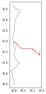
Fig. 54 Solution of exercise-08-d2: Routes by "מטרופולין" with maximal delta_lon and delta_lat (plot)