
Geometric operations
Contents
Geometric operations#
Last updated: 2023-02-25 13:41:03
Introduction#
In the previous chapter we introduced the geopandas package, focusing on non-spatial operations such as subsetting by attributes (see Filtering by attributes), as well as geometry-related transformations (see Table to point layer and Points to line (geopandas)).
In this chapter, we go further into operations that involve the geometric component of one or more GeoDataFrame vector layer, using the geopandas package. This group of operations includes the following standard spatial analysis functions:
CRS and reprojection—Transforming a given layer from one CRS to another
Numeric calculations—Calculating numeric geometry properties, such as length, area, and distance
New geometries—Creating new geometries, such as calculating buffers, or area of intersection
Geometric relations—Evaluating the relation between layers, such as whether two geometries intersect
Spatial join—Joining attributes from one layer to another, based on spatial relations
By the end of this chapter, you will have an overview of all common worflows in spatial analysis of vector layers.
Sample data#
Overview#
First, let us prepare the environment to demostrate geometric operations using geopandas. First, we load the geopandas package:
import geopandas as gpd
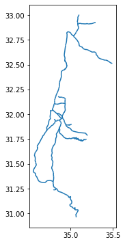
Next, let us load three layers, subset the relevant columns, and examine them visually. The first two (towns and rail) are familiar from the previous chapter (see Reading vector layers), while the third one (stations) is new:
towns—A polygonal layer of towns (see Towns)rail—A line layer of railway lines (see Railway lines)stations—A point layer of railway stations (see Railway stations)
Towns#
The polygonal towns layer is imported from the Shapefile named muni_il.shp. Then we select four attributes of interest (and the "geometry" column):
towns = gpd.read_file('data/muni_il.shp', encoding='utf-8')
towns = towns[['Muni_Heb', 'Machoz', 'Shape_Area', 'geometry']]
towns
| Muni_Heb | Machoz | Shape_Area | geometry | |
|---|---|---|---|---|
| 0 | ללא שיפוט - אזור מעיליא | צפון | 2.001376e+05 | POLYGON Z ((225369.655 770523.6... |
| 1 | תמר | דרום | 1.597418e+09 | POLYGON Z ((206899.135 552967.8... |
| 2 | שהם | מרכז | 6.177438e+06 | POLYGON Z ((194329.250 655299.1... |
| 3 | שהם | מרכז | 9.850450e+05 | POLYGON Z ((196236.573 657835.0... |
| 4 | ראש פינה | צפון | 6.104233e+04 | POLYGON Z ((255150.135 764764.6... |
| ... | ... | ... | ... | ... |
| 405 | אופקים | דרום | 1.635240e+07 | POLYGON Z ((164806.146 577898.8... |
| 406 | אבן יהודה | מרכז | 8.141962e+06 | POLYGON Z ((189803.359 684152.9... |
| 407 | אבו סנאן | צפון | 6.455340e+06 | POLYGON Z ((212294.953 763168.8... |
| 408 | אבו גוש | ירושלים | 1.891242e+06 | POLYGON Z ((209066.649 635655.2... |
| 409 | שדות נגב | דרום | 2.554627e+05 | POLYGON Z ((162082.027 592043.1... |
410 rows × 4 columns
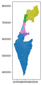
Here is the towns layer, colored by the "Machoz" administrative division:
towns.plot(column='Machoz');
Railway lines#
Next, we read the railway line layer, from the Shapefile named RAIL_STRATEGIC.shp. We subset the layer by attributes (see Filtering by attributes) to retain just the active railway segments. Then, we subset just the "SEGMENT" (segment name) and "geometry" columns:
rail = gpd.read_file('data/RAIL_STRATEGIC.shp')
rail = rail[rail['ISACTIVE'] == 'פעיל']
rail = rail[['SEGMENT', 'geometry']]
rail
| SEGMENT | geometry | |
|---|---|---|
| 0 | כפר יהושע - נשר_1 | LINESTRING (205530.083 741562.9... |
| 1 | באר יעקב-ראשונים_2 | LINESTRING (181507.598 650706.1... |
| 3 | לב המפרץ מזרח - נשר_4 | LINESTRING (203482.789 744181.5... |
| 4 | קרית גת - להבים_5 | LINESTRING (178574.101 609392.9... |
| 5 | רמלה - רמלה מזרח_6 | LINESTRING (189266.580 647211.5... |
| ... | ... | ... |
| 210 | ויתקין - חדרה_215 | LINESTRING (190758.230 704950.0... |
| 211 | בית יהושע - נתניה ספיר_216 | LINESTRING (187526.597 687360.3... |
| 214 | השמונה - בית המכס_220 | LINESTRING (200874.999 746209.3... |
| 215 | לב המפרץ - בית המכס_221 | LINESTRING (203769.786 744358.6... |
| 216 | 224_לוד מרכז - נתבג | LINESTRING (190553.481 654170.3... |
161 rows × 2 columns
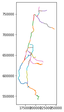
Here is a plot of the rail layer, colored by segment name:
rail.plot(column='SEGMENT');
Railway stations#
Finally, we read a layer of rainway stations, from a Shapefile named RAIL_STAT_ONOFF_MONTH.shp. The attributes of interest which we retain (in addition to the "geometry") are:
"STAT_NAMEH"—Station name"ON_7_DAY"—Passengers entering the station at 7:00-8:00 during September 2020"OFF_7_DAY"—Passengers exiting the station at 7:00-8:00 during September 2020"ON_17_DAY"—Passengers entering the station at 17:00-18:00 during September 2020"OFF_17_DAY"—Passengers exiting the station at 17:00-18:00 during September 2020
stations = gpd.read_file('data/RAIL_STAT_ONOFF_MONTH.shp')
stations = stations[['STAT_NAMEH', 'ON_7_DAY', 'OFF_7_DAY', 'ON_17_DAY', 'OFF_17_DAY', 'geometry']]
stations
| STAT_NAMEH | ON_7_DAY | OFF_7_DAY | ON_17_DAY | OFF_17_DAY | geometry | |
|---|---|---|---|---|---|---|
| 0 | ראשון לציון משה דיין | 129.0 | 72.0 | 71.0 | 123.0 | POINT (177206.094 655059.936) |
| 1 | קרית ספיר נתניה | 34.0 | 119.0 | 120.0 | 40.0 | POINT (187592.123 687587.598) |
| 2 | ת"א השלום | 158.0 | 1642.0 | 2091.0 | 355.0 | POINT (180621.940 664537.210) |
| 3 | שדרות | 80.0 | 26.0 | 24.0 | 79.0 | POINT (160722.849 602798.889) |
| 4 | רמלה | 140.0 | 47.0 | 34.0 | 87.0 | POINT (188508.910 648466.870) |
| ... | ... | ... | ... | ... | ... | ... |
| 58 | מגדל העמק כפר ברוך | 21.0 | 5.0 | 8.0 | 24.0 | POINT (219851.931 728164.825) |
| 59 | באר שבע אוניברסיטה | 212.0 | 130.0 | 89.0 | 184.0 | POINT (181813.614 574550.411) |
| 60 | חיפה בת גלים | 106.0 | 311.0 | 108.0 | 68.0 | POINT (198610.010 748443.790) |
| 61 | לוד | 321.0 | 238.0 | 198.0 | 297.0 | POINT (188315.977 650289.373) |
| 62 | נהריה | 0.0 | 64.0 | 0.0 | 326.0 | POINT (209570.590 767769.220) |
63 rows × 6 columns
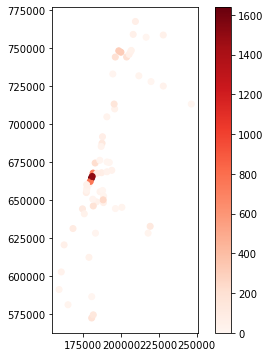
Here is a visualization of the stations layer. Using symbology, we demonstrate that the largest number of passengers exiting a station in 7:00-8:00 are in Tel-Aviv, where lots of people travel to work:
stations.plot(column='OFF_7_DAY', cmap='Reds', legend=True);
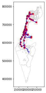
Here is the plot of the towns, stations, and rail layers, together (see Plotting more than one layer):
base = towns.plot(color='white', edgecolor='lightgrey')
stations.plot(ax=base, color='red')
rail.plot(ax=base, color='blue');
CRS and reprojection#
What is a CRS?#
A Coordinate Reference System (CRS) defines the association between coordinates (which are ultimately just numbers) and specific locations on the surface of the earth. CRS can be divided into two groups:
Geographic CRS, where units are degrees (e.g., WGS84)
Projected CRS, where using are “real” distance units, typically meters (e.g., ITM, UTM)
There are several methods and formats to describe and specify a CRS. The shortest and simplest method is to use an EPSG code, which all standard CRS have. For example, Table 23 specifies the CRS we encounter in this book, and their EPSG codes.
Name |
Type |
Units |
EPSG code |
|---|---|---|---|
WGS84 |
Geographic |
Degrees |
|
ITM |
Projected |
Meters |
|
UTM Zone 36N |
Projected |
Meters |
|
Geographic CRS refer to the entire surface of the Earth, while projected CRS commonly refer to smaller areas. A fundamental difference between geographical and projected CRS is in their units. Geographic CRS refer to location on a sphere, using degree units, while projected CRS refer to locations on an approximated planar surface. One important implication of the unit difference is that planar gemetric calculations (such as distance and area) make sense in projected CRS, but not in geographic CRS.
Note
There are several formats, or standards, to specify a CRS, in Python and elsewhere. The most common ones are:
An EPSG code (such as
4326)A PROJ string (such as
"+proj=longlat +datum=WGS84 +no_defs")A WKT string (such as
"GEOGCS["WGS 84",DATUM["WGS_1984",...[etc.]")
In this book, we exclusively use EPSG codes to define projections, for their simplicity.
Examining with .crs#
As mentioned previously, the CRS definition of a GeoDataFrame (or a GeoSeries) is accessible through the .crs property (see GeoDataFrame structure). For example, here is the CRS information of the rail layer:
rail.crs
<Derived Projected CRS: EPSG:2039>
Name: Israel 1993 / Israeli TM Grid
Axis Info [cartesian]:
- E[east]: Easting (metre)
- N[north]: Northing (metre)
Area of Use:
- name: Israel - onshore; Palestine Territory - onshore.
- bounds: (34.17, 29.45, 35.69, 33.28)
Coordinate Operation:
- name: Israeli TM
- method: Transverse Mercator
Datum: Israel 1993
- Ellipsoid: GRS 1980
- Prime Meridian: Greenwich
The rail layer is in the ITM system. The EPSG code of this CRS is 2039. Exploring the printout can also reveal that the CRS units are meters, and that the geographical area where the CRS is supposed to be used is Israel.
Modifying with .set_crs#
To modify the CRS definition of a given layer, we can use the .set_crs method. In case the layer already has a CRS definition, we must use the allow_override=True option. Otherwise, we get an error. The allow_override argument is a safeguard against replacing the CRS definition of a layer when it already has one, which only makes sense if the existing CRS definition is wrong and we need to “fix” it (see below).
For example, the following expression replaces the CRS definition of rail (which is ITM, 2039) with another CRS (WGS84, 4326):
rail = rail.set_crs(4326, allow_override=True)
We can examine the .crs property, to see that the CRS definition has indeed changed:
rail.crs
<Geographic 2D CRS: EPSG:4326>
Name: WGS 84
Axis Info [ellipsoidal]:
- Lat[north]: Geodetic latitude (degree)
- Lon[east]: Geodetic longitude (degree)
Area of Use:
- name: World.
- bounds: (-180.0, -90.0, 180.0, 90.0)
Datum: World Geodetic System 1984 ensemble
- Ellipsoid: WGS 84
- Prime Meridian: Greenwich
It is important to note that replacing the CRS definition has no effect on the coordinates. For example, the coordinates of rail are still in ITM units, rather than decimal degrees:
print(rail['geometry'].iloc[11])
LINESTRING (188700.04908514675 648249.5428679045, 188521.65428514872 648456.553667903)
This means that the layer is now incorrect (!), since the coordinates do not match the CRS definition. Replacing the CRS definition should only be done when:
The layer has no CRS definition, e.g., it was accidentally lost, and we need to restore it
The CRS definition is incorrect, and we need to replace it
Let us now modify the CRS definition back to the original, to “fix” the layer we have just broken:
rail = rail.set_crs(2039, allow_override=True)
Note
To remove the CRS definition of a given layer altogether, you can assign None to the .crs property, as in rail.crs=None.
Reprojecting with .to_crs#
Reprojecting a vector layer involves not just replacing the CRS definition (see Modifying with .set_crs), but also re-calculating all of the layer coordinates, so that they are in agreement with the new CRS.
To reproject a GeoDataFrame, or a GeoSeries, we use the .to_crs method. For example, here is how we can transform the rail layer to WGS84:
rail = rail.to_crs(4326)
Comparing the updated .crs property of rail with the original one (see above), we can see that the CRS definition indeed changed:
rail.crs
<Geographic 2D CRS: EPSG:4326>
Name: WGS 84
Axis Info [ellipsoidal]:
- Lat[north]: Geodetic latitude (degree)
- Lon[east]: Geodetic longitude (degree)
Area of Use:
- name: World.
- bounds: (-180.0, -90.0, 180.0, 90.0)
Datum: World Geodetic System 1984 ensemble
- Ellipsoid: WGS 84
- Prime Meridian: Greenwich
Importantly, the coordinates also changed, which can be demonstrated by printing the WKT representation of any given geometry from the layer (compare with the above printout):
print(rail['geometry'].iloc[11])
LINESTRING (34.87921676021756 31.926817568737928, 34.87732378978819 31.928679560071494)
Thus the information in the rail layer is still “correct”, as the coordinates match the CRS. It is just in a different CRS.
Finally, we can see that the axis text labels when plotting the layer have changed, now reflecting decimal degree values of the WGS84 CRS:
rail.plot();
Let us reproject rail back to the original CRS (i.e., ITM) before we proceed:
rail = rail.to_crs(epsg=2039)
Note
More information on specifying projections, and reprojecting layers, can be found in https://geopandas.org/docs/user_guide/projections.html.
Numeric calculations#
Overview#
In this section, we cover geometric commonly used calculations that result in numeric values, using geopandas. As we will see, the first three operations are very similar to their shapely counterparts (Table 24). The principle difference is that the calculation is applied on multiple geometries, rather than just one.
Method |
|
|
|---|---|---|
|
see Length (shapely) |
|
|
see Area (shapely) |
see Area (geopandas) |
|
The fourth operation, detecting nearest neighbors (see Nearest neighbors), is a little more complex and not really analogous to any shapely-based workflow, since it only makes sense to detect nearest neighbors when we have more than one geometry to choose from.
Length (geopandas)#
The .length property returns a Series with line lengths per geometry in a GeoDataFrame (or a GeoSeries). For example, rail.length returns a Series of railway segment lengths:
rail.length
0      12379.715331
1       2274.111799
3       2793.337699
4       1960.170882
5       1195.701220
           ...
210     5975.045997
211     1913.384027
214     1603.616014
215      166.180958
216     1284.983680
Length: 161, dtype: float64
Keep in mind that all numeric calculations, such as length, area (see Area (geopandas)), and distance (see Distance (geopandas)), are returned in the coordinate units, that is, in CRS units. In our case, the CRS is ITM, where the units are meters (\(m\)) (Table 23). The following expression transforms the values from \(m\) to \(km\):
rail.length / 1000
0      12.379715
1       2.274112
3       2.793338
4       1.960171
5       1.195701
         ...
210     5.975046
211     1.913384
214     1.603616
215     0.166181
216     1.284984
Length: 161, dtype: float64
This Series can be assigned to into a new column, such as a column named "length_km", as follows:
rail['length_km'] = rail.length / 1000
rail
| SEGMENT | geometry | length_km | |
|---|---|---|---|
| 0 | כפר יהושע - נשר_1 | LINESTRING (205530.083 741562.9... | 12.379715 |
| 1 | באר יעקב-ראשונים_2 | LINESTRING (181507.598 650706.1... | 2.274112 |
| 3 | לב המפרץ מזרח - נשר_4 | LINESTRING (203482.789 744181.5... | 2.793338 |
| 4 | קרית גת - להבים_5 | LINESTRING (178574.101 609392.9... | 1.960171 |
| 5 | רמלה - רמלה מזרח_6 | LINESTRING (189266.580 647211.5... | 1.195701 |
| ... | ... | ... | ... |
| 210 | ויתקין - חדרה_215 | LINESTRING (190758.230 704950.0... | 5.975046 |
| 211 | בית יהושע - נתניה ספיר_216 | LINESTRING (187526.597 687360.3... | 1.913384 |
| 214 | השמונה - בית המכס_220 | LINESTRING (200874.999 746209.3... | 1.603616 |
| 215 | לב המפרץ - בית המכס_221 | LINESTRING (203769.786 744358.6... | 0.166181 |
| 216 | 224_לוד מרכז - נתבג | LINESTRING (190553.481 654170.3... | 1.284984 |
161 rows × 3 columns
All geometric operations in geopandas assume planar geometry, returning the result in the CRS units. This means that layers in a geographic CRS (such as WGS84) need to be transformed to a projected CRS (see What is a CRS?) before any geometric calculation. Otherwise, numeric measurements, such as length, area, and distance, are going to be returned in decimal degree units, which usually does not make sense, as the relation between degrees and geographic distance is not a fixed one.
Exercise 09-a
Reproject the
raillayer to geographic coordinates (4326), than calculate railway lengths once again. You should see the (meaningless) results in decimal degrees.
Area (geopandas)#
The .area property returns a Series with the area per geometry in a GeoDataFrame (or a GeoSeries). For example, towns.area returns the area sizes of each polygon in the towns layer, again in CRS units (\(m^2\)):
towns.area
0      2.001376e+05
1      1.597418e+09
2      6.177438e+06
3      9.850450e+05
4      6.104233e+04
           ...
405    1.635240e+07
406    8.141962e+06
407    6.455340e+06
408    1.891242e+06
409    2.554627e+05
Length: 410, dtype: float64
If necessary, this series can be assigned to a new column. For example, the following expression divides the area values by a factor of \(1000^2\), i.e., 1000**2 to convert from \(m^2\) to \(km^2\), then assigns the results to a new column named "area_km2":
towns['area_km2'] = towns.area / 1000**2
towns
| Muni_Heb | Machoz | Shape_Area | geometry | area_km2 | |
|---|---|---|---|---|---|
| 0 | ללא שיפוט - אזור מעיליא | צפון | 2.001376e+05 | POLYGON Z ((225369.655 770523.6... | 0.200138 |
| 1 | תמר | דרום | 1.597418e+09 | POLYGON Z ((206899.135 552967.8... | 1597.417603 |
| 2 | שהם | מרכז | 6.177438e+06 | POLYGON Z ((194329.250 655299.1... | 6.177438 |
| 3 | שהם | מרכז | 9.850450e+05 | POLYGON Z ((196236.573 657835.0... | 0.985045 |
| 4 | ראש פינה | צפון | 6.104233e+04 | POLYGON Z ((255150.135 764764.6... | 0.061042 |
| ... | ... | ... | ... | ... | ... |
| 405 | אופקים | דרום | 1.635240e+07 | POLYGON Z ((164806.146 577898.8... | 16.352399 |
| 406 | אבן יהודה | מרכז | 8.141962e+06 | POLYGON Z ((189803.359 684152.9... | 8.141962 |
| 407 | אבו סנאן | צפון | 6.455340e+06 | POLYGON Z ((212294.953 763168.8... | 6.455340 |
| 408 | אבו גוש | ירושלים | 1.891242e+06 | POLYGON Z ((209066.649 635655.2... | 1.891242 |
| 409 | שדות נגב | דרום | 2.554627e+05 | POLYGON Z ((162082.027 592043.1... | 0.255463 |
410 rows × 5 columns
Exercise 09-b
Find out the names of the largest and the smallest municipal area polygon, in terms of area size, based on the
townslayer. (answer:'ללא שיפוט - אזור נחל ארבל'and'רמת נגב')
Exercise 09-c
Check the association between the
"area"column we calculated, and the"Shape_Area"column which is stored in the Shapefile, using a scatterplot (see Scatterplots (pandas)) (Fig. 55).
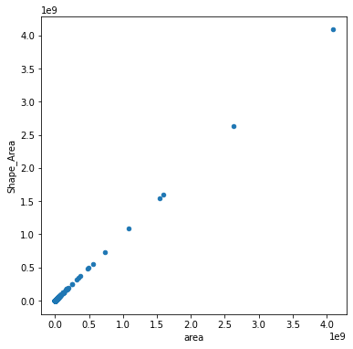
Fig. 55 Solution of exercise-09-c: Association between the (calculated) "area" column and the (original) "Shape_Area" column#
Distance (geopandas)#
The .distance method can be used to calculate distances. This method can be used to calculate pairwise distances between two GeoSeries (aligned by index or position), or between each geometry in one GeoSeries and another, individual, geometry. The following example demonstrates the latter. Here, we are calculating the distances between:
stations—all railway stations, andrail['geometry'].iloc[0]—the first railway segment.
The result is a Series of distances, in \(m\):
stations.distance(rail['geometry'].iloc[0])
0      84284.975205
1      50424.920267
2      74235.170679
3     138847.580690
4      86603.473121
          ...
58      8595.362486
59    160138.041969
60      9758.724335
61     84904.898970
62     26515.877484
Length: 63, dtype: float64
What if we need to calculate the pairwise distances, between each station and each railway segment? This can be done using .apply (see apply and custom functions). The following expression, in plain language, means that we take each row (axis=1) in stations as x, then calculate the Series of distances from all railway segments to the geometry of that row (rail.distance(x["geometry"])).
The result is a DataFrame representing a distance matrix, where:
Rows represent railway stations
Columns represent railway segments
Cell values are distances, in meters
d = stations.apply(lambda x: rail.distance(x['geometry']), axis=1)
d
| 0 | 1 | 3 | 4 | 5 | ... | 210 | 211 | 214 | 215 | 216 | |
|---|---|---|---|---|---|---|---|---|---|---|---|
| 0 | 84284.975205 | 6120.325293 | 91266.392666 | 43769.104489 | 13360.106887 | ... | 46002.039665 | 31998.139305 | 94172.402848 | 93091.940077 | 13376.996382 |
| 1 | 50424.920267 | 37379.975682 | 57120.870160 | 76795.773036 | 39353.653794 | ... | 11924.365438 | 236.552504 | 60107.821537 | 58958.887738 | 33548.162167 |
| 2 | 74235.170679 | 13859.386195 | 81199.631964 | 53259.279461 | 18180.867522 | ... | 35958.589113 | 21932.455984 | 84145.901064 | 83037.130172 | 14356.406044 |
| 3 | 138847.580690 | 51367.336965 | 146064.901194 | 19030.199927 | 52794.173376 | ... | 100790.724935 | 86796.547920 | 148925.381315 | 147885.212962 | 58403.590869 |
| 4 | 86603.473121 | 5697.560021 | 94960.212976 | 38438.916853 | 289.422152 | ... | 50857.456340 | 37074.116175 | 98521.682411 | 97044.665341 | 4964.211497 |
| ... | ... | ... | ... | ... | ... | ... | ... | ... | ... | ... | ... |
| 58 | 8595.362486 | 86339.689331 | 20244.761995 | 123902.486603 | 85772.327241 | ... | 37220.552915 | 52057.048736 | 26186.457201 | 22822.683088 | 79583.761529 |
| 59 | 160138.041969 | 74611.504901 | 169029.718846 | 34992.788653 | 73042.322269 | ... | 125012.376699 | 111083.909066 | 172714.053593 | 171172.498821 | 78870.029306 |
| 60 | 9758.724335 | 99222.671750 | 6473.850217 | 138574.693149 | 100683.138956 | ... | 44196.792329 | 62080.870950 | 1709.845960 | 6471.883040 | 94617.022408 |
| 61 | 84904.898970 | 5579.557103 | 93200.557041 | 40156.246177 | 2075.672842 | ... | 49040.957113 | 35245.583872 | 96738.721423 | 95275.546196 | 3553.733949 |
| 62 | 26515.877484 | 120379.789258 | 24360.621700 | 159481.427917 | 121328.202345 | ... | 65575.558369 | 83375.846025 | 22375.584322 | 24118.556926 | 115179.615344 |
63 rows × 161 columns
Note that the first column in the above result is identical to the Series we got in the previous expression.
The distance matrix can be refined to calculate more specific properties related to distance that we are interested in. For example, to get the minimum distance to any of the railway segments (rather than all distances), we can apply the .min() method on each row, as follows. The result is a Series of minimal distances per station:
nearest_seg_dist = d.min(axis=1)
nearest_seg_dist
0      13.440327
1       4.932094
2      16.180832
3      64.381044
4       2.941401
         ...
58     56.102377
59      7.540327
60     44.130049
61     22.556829
62    115.502833
Length: 63, dtype: float64
We can assign it to a new column named "nearest_seg_dist" (“distance to nearest segment”) in stations, as follows:
stations['nearest_seg_dist'] = nearest_seg_dist
stations
| STAT_NAMEH | ON_7_DAY | OFF_7_DAY | ON_17_DAY | OFF_17_DAY | geometry | nearest_seg_dist | |
|---|---|---|---|---|---|---|---|
| 0 | ראשון לציון משה דיין | 129.0 | 72.0 | 71.0 | 123.0 | POINT (177206.094 655059.936) | 13.440327 |
| 1 | קרית ספיר נתניה | 34.0 | 119.0 | 120.0 | 40.0 | POINT (187592.123 687587.598) | 4.932094 |
| 2 | ת"א השלום | 158.0 | 1642.0 | 2091.0 | 355.0 | POINT (180621.940 664537.210) | 16.180832 |
| 3 | שדרות | 80.0 | 26.0 | 24.0 | 79.0 | POINT (160722.849 602798.889) | 64.381044 |
| 4 | רמלה | 140.0 | 47.0 | 34.0 | 87.0 | POINT (188508.910 648466.870) | 2.941401 |
| ... | ... | ... | ... | ... | ... | ... | ... |
| 58 | מגדל העמק כפר ברוך | 21.0 | 5.0 | 8.0 | 24.0 | POINT (219851.931 728164.825) | 56.102377 |
| 59 | באר שבע אוניברסיטה | 212.0 | 130.0 | 89.0 | 184.0 | POINT (181813.614 574550.411) | 7.540327 |
| 60 | חיפה בת גלים | 106.0 | 311.0 | 108.0 | 68.0 | POINT (198610.010 748443.790) | 44.130049 |
| 61 | לוד | 321.0 | 238.0 | 198.0 | 297.0 | POINT (188315.977 650289.373) | 22.556829 |
| 62 | נהריה | 0.0 | 64.0 | 0.0 | 326.0 | POINT (209570.590 767769.220) | 115.502833 |
63 rows × 7 columns
Nearest neighbors#
Here is another technique to extract information from the distance matrix, expanding the above expression of distance to nearest neighbor. This time, we calculate the name ("SEGMENT" column) of the nearest railway segment for each station. We are using the .idxmin method (see Table 15), instead of .min, to get the index of the nearest segment (instead of the distance to it):
d.idxmin(axis=1)
0      22
1     100
2      57
3     131
4      87
     ...
58    152
59    205
60    153
61     77
62     12
Length: 63, dtype: int64
The index can then be used to subset segment names (rail["SEGMENT"]). The result is a series of the nearest segment names:
nearest_seg_name = rail['SEGMENT'].loc[d.idxmin(axis=1)]
nearest_seg_name
22              משה דיין-קוממיות_23
100    נתניה מכללה - נתניה ספיר_101
57           סבידור מרכז - השלום_58
131              שדרות-יד מרדכי_134
87                    לוד - רמלה_88
                   ...
152            עפולה - כפר ברוך_155
205    באר שבע צפון - באר שבע אוניב
153          חוף כרמל - בת גלים_156
77                    לוד - רמלה_78
12                   נהריה - עכו_13
Name: SEGMENT, Length: 63, dtype: object
Let us attach the result to another column in the stations table, named nearest_seg_name (“nearest segment name”). We need to reset the indices to make sure the column is attached by position:
nearest_seg_name = nearest_seg_name.reset_index(drop=True)
nearest_seg_name
0              משה דיין-קוממיות_23
1     נתניה מכללה - נתניה ספיר_101
2           סבידור מרכז - השלום_58
3               שדרות-יד מרדכי_134
4                    לוד - רמלה_88
                  ...
58            עפולה - כפר ברוך_155
59    באר שבע צפון - באר שבע אוניב
60          חוף כרמל - בת גלים_156
61                   לוד - רמלה_78
62                  נהריה - עכו_13
Name: SEGMENT, Length: 63, dtype: object
stations['nearest_seg_name'] = nearest_seg_name
stations
| STAT_NAMEH | ON_7_DAY | OFF_7_DAY | ON_17_DAY | OFF_17_DAY | geometry | nearest_seg_dist | nearest_seg_name | |
|---|---|---|---|---|---|---|---|---|
| 0 | ראשון לציון משה דיין | 129.0 | 72.0 | 71.0 | 123.0 | POINT (177206.094 655059.936) | 13.440327 | משה דיין-קוממיות_23 |
| 1 | קרית ספיר נתניה | 34.0 | 119.0 | 120.0 | 40.0 | POINT (187592.123 687587.598) | 4.932094 | נתניה מכללה - נתניה ספיר_101 |
| 2 | ת"א השלום | 158.0 | 1642.0 | 2091.0 | 355.0 | POINT (180621.940 664537.210) | 16.180832 | סבידור מרכז - השלום_58 |
| 3 | שדרות | 80.0 | 26.0 | 24.0 | 79.0 | POINT (160722.849 602798.889) | 64.381044 | שדרות-יד מרדכי_134 |
| 4 | רמלה | 140.0 | 47.0 | 34.0 | 87.0 | POINT (188508.910 648466.870) | 2.941401 | לוד - רמלה_88 |
| ... | ... | ... | ... | ... | ... | ... | ... | ... |
| 58 | מגדל העמק כפר ברוך | 21.0 | 5.0 | 8.0 | 24.0 | POINT (219851.931 728164.825) | 56.102377 | עפולה - כפר ברוך_155 |
| 59 | באר שבע אוניברסיטה | 212.0 | 130.0 | 89.0 | 184.0 | POINT (181813.614 574550.411) | 7.540327 | באר שבע צפון - באר שבע אוניב |
| 60 | חיפה בת גלים | 106.0 | 311.0 | 108.0 | 68.0 | POINT (198610.010 748443.790) | 44.130049 | חוף כרמל - בת גלים_156 |
| 61 | לוד | 321.0 | 238.0 | 198.0 | 297.0 | POINT (188315.977 650289.373) | 22.556829 | לוד - רמלה_78 |
| 62 | נהריה | 0.0 | 64.0 | 0.0 | 326.0 | POINT (209570.590 767769.220) | 115.502833 | נהריה - עכו_13 |
63 rows × 8 columns
The last example can be considered as a “manually” constructed nearest-neighbor spatial join, since we actually joined an attribute ("SEGMENT") value from one layer (rail) to another layer (stations), based on proximity. Towards the end of this chapter we will introduce the the gpd.sjoin_nearest function which can be used for nearest-neighbour spatial join using much shorter code (see Nearest neighbor join).
New geometries#
Overview#
In this section, we learn about functions that calculate new geometries. We are already familiar with the analogous operation for individual geometries (see New geometries 1 and New geometries 2). Now, we learn about the same type of operations for layers, which include more than one geometry. In general, the operation is repeated for each geometry, or each pair of geometries, resulting in a new geometry column with the results. For example, when applying a “centroid” function on a vector layer or geometry column, we get a new geometry column, with the same number of geometries as the original, where each geometry is the centroid of the respective original geometry.
Just like when discussing the shapely functions, we can distinguish between functions that accept a single layer (see Centroids (geopandas) and Buffers (geopandas)) and functions that accept a pair of layers (see Set-operations (.overlay)). The first two methods (.centroid and .buffer) are very similar in shapely and geopandas. Creating new geometries based on pairs of input geometries, however, is different (Table 25):
In
shapely, there are specific functions for each pairwise algorithm (.intersection,.union,.difference) (see New geometries 2)In
geopandas, there is one method (.overlay) where the algorithm is specified using thehowargument (see Set-operations (.overlay))
Method |
|
|
|---|---|---|
|
||
|
||
|
||
|
||
|
Note
geopandas also has the .intersection, .union, and .difference methods, but these operate on the geometric part of the vector layer only (the GeoSeries). Therefore, they do not preserve the attribute data, which is rarely what we want.
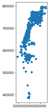
Centroids (geopandas)#
The .centroid method, applied on a GeoDataFrame or GeoSeries, returns a new GeoSeries with the centroids. For example, here is how we can create a GeoSeries of town polygon centroids:
ctr = towns.centroid
ctr
0      POINT (225182.898 770809.745)
1      POINT (228716.918 561880.946)
2      POINT (195454.340 655942.058)
3      POINT (196351.843 658288.230)
4      POINT (254877.752 764800.811)
                   ...
405    POINT (165198.012 579543.277)
406    POINT (189227.026 686069.086)
407    POINT (215379.077 763146.384)
408    POINT (210369.545 634906.185)
409    POINT (161682.995 591763.635)
Length: 410, dtype: geometry
And here is a plot of the result:
ctr.plot();
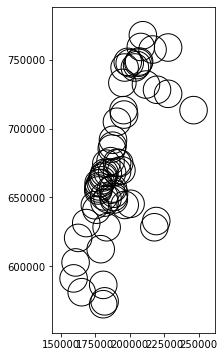
Buffers (geopandas)#
The .buffer method buffers each geometry in a given GeoDataFrame or GeoSeries to the specified distance. It returns a GeoSeries with the resulting polygons. For example, here we create buffers of 10,000 \(m\) (i.e., 10 \(km\)) around each railway station:
stations_buffer = stations.buffer(10000)
stations_buffer
0     POLYGON ((187206.094 655059.936...
1     POLYGON ((197592.123 687587.598...
2     POLYGON ((190621.940 664537.210...
3     POLYGON ((170722.849 602798.889...
4     POLYGON ((198508.910 648466.870...
                     ...
58    POLYGON ((229851.931 728164.825...
59    POLYGON ((191813.614 574550.411...
60    POLYGON ((208610.010 748443.790...
61    POLYGON ((198315.977 650289.373...
62    POLYGON ((219570.590 767769.220...
Length: 63, dtype: geometry
Here is a plot of the result:
stations_buffer.plot(color='none');
Exercise 09-d
As shown above, centroids and buffers are returned as a
GeoSeries.Suppose that, instead, you need a
GeoDataFramewith the original attributes of the source layer (e.g., the railway station properties) and the centroid, or buffer, geometries. How can we create suchGeoDataFrames?
Set-operations (.overlay)#
We can apply set operations on geometry pairs, using the .overlay method, to obtain a new layer of the results. For example, x.overlay(y,how="intersection") returns all the intersections between a feature in x and a feature in y. The .overlay method supports the same pairwise set operations that shapely does (see New geometries 2), such as intersection or union. The principal difference is that we are executing the operation on a multple pairs of geometries, coming from two layers, rather than just two individual geometries. Accordingly, we get back a layer with the pairwise results. In other words, the operation is executed for each combination of one geometry taken from the first series and one geometry taken from the other series.
The how argument of .overlay specifies the type of the set operation. It can be one of:
"intersection"(the default)"union""difference""symmetric_difference""identity"
For example, the following expression calculates the pairwise intersections between railway segments (rail) and towns (towns), creating a new layer of pairwise intersections rail_towns:
rail_towns = rail[['SEGMENT', 'length_km', 'geometry']].overlay(towns[['Muni_Heb', 'geometry']])
rail_towns
---------------------------------------------------------------------------
ImportError                               Traceback (most recent call last)
/tmp/ipykernel_13095/1365625897.py in <module>
----> 1 rail_towns = rail[['SEGMENT', 'length_km', 'geometry']].overlay(towns[['Muni_Heb', 'geometry']])
      2 rail_towns

~/.local/lib/python3.10/site-packages/geopandas/geodataframe.py in overlay(self, right, how, keep_geom_type, make_valid)
   2350         dimension is not taken into account.
   2351         """
-> 2352         return geopandas.overlay(
   2353             self, right, how=how, keep_geom_type=keep_geom_type, make_valid=make_valid
   2354         )

~/.local/lib/python3.10/site-packages/geopandas/tools/overlay.py in overlay(df1, df2, how, keep_geom_type, make_valid)
    315             result = _overlay_difference(df1, df2)
    316         elif how == "intersection":
--> 317             result = _overlay_intersection(df1, df2)
    318         elif how == "symmetric_difference":
    319             result = _overlay_symmetric_diff(df1, df2)

~/.local/lib/python3.10/site-packages/geopandas/tools/overlay.py in _overlay_intersection(df1, df2)
     28     """
     29     # Spatial Index to create intersections
---> 30     idx1, idx2 = df2.sindex.query_bulk(df1.geometry, predicate="intersects", sort=True)
     31     # Create pairs of geometries in both dataframes to be intersected
     32     if idx1.size > 0 and idx2.size > 0:

~/.local/lib/python3.10/site-packages/geopandas/base.py in sindex(self)
   2704                [2]])
   2705         """
-> 2706         return self.geometry.values.sindex
   2707
   2708     @property

~/.local/lib/python3.10/site-packages/geopandas/array.py in sindex(self)
    289     def sindex(self):
    290         if self._sindex is None:
--> 291             self._sindex = _get_sindex_class()(self.data)
    292         return self._sindex
    293

~/.local/lib/python3.10/site-packages/geopandas/sindex.py in _get_sindex_class()
     19     if compat.HAS_RTREE:
     20         return RTreeIndex
---> 21     raise ImportError(
     22         "Spatial indexes require either `rtree` or `pygeos`. "
     23         "See installation instructions at https://geopandas.org/install.html"

ImportError: Spatial indexes require either `rtree` or `pygeos`. See installation instructions at https://geopandas.org/install.html
To understand what has happened, consider a specific segment in the rail layer:
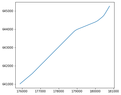
x = rail[rail['SEGMENT'] == 'רחובות גבירול-יבנה מזרח_53']
x
| SEGMENT | geometry | length_km | |
|---|---|---|---|
| 52 | רחובות גבירול-יבנה מזרח_53 | LINESTRING (175871.680 640999.6... | 6.611288 |
Here is a plot of this particular segment:
x.plot();
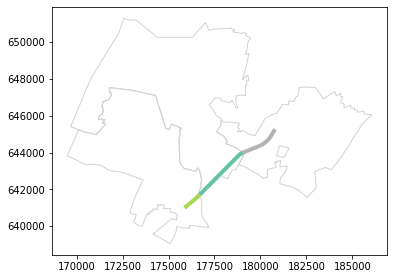
In the result of the overlay operation, this segment was split into three parts, since it crosses three different geometries from the towns layer. We can see, in the result, the names of the towns feature that the sub- railway segment crosses:
y = rail_towns[rail_towns['SEGMENT'] == 'רחובות גבירול-יבנה מזרח_53']
y
| SEGMENT | length_km | Muni_Heb | geometry | |
|---|---|---|---|---|
| 82 | רחובות גבירול-יבנה מזרח_53 | 6.611288 | יבנה | LINESTRING Z (175871.680 640999... |
| 85 | רחובות גבירול-יבנה מזרח_53 | 6.611288 | גן רוה | LINESTRING Z (176705.464 641722... |
| 134 | רחובות גבירול-יבנה מזרח_53 | 6.611288 | רחובות | LINESTRING Z (179037.308 643998... |
as demonstrated in the following plot:
base = towns[towns['Muni_Heb'].isin(y['Muni_Heb'])].plot(color='none', edgecolor='lightgrey', zorder=1)
y.plot(ax=base, column='Muni_Heb', cmap='Set2', linewidth=4, zorder=2);
Note that the length attribute was “inherited” from the original rail layer, and it no longer represents the length of the sub-segments resulting from the overlay operation. If necessary, we can “update” the length attribute by recalculating geometry lengths:
rail_towns['length_km'] = rail_towns.length / 1000
Now the "length_km" attribute in rail_towns is correct:
rail_towns[rail_towns['SEGMENT'] == 'רחובות גבירול-יבנה מזרח_53']
| SEGMENT | length_km | Muni_Heb | geometry | |
|---|---|---|---|---|
| 82 | רחובות גבירול-יבנה מזרח_53 | 1.104030 | יבנה | LINESTRING Z (175871.680 640999... |
| 85 | רחובות גבירול-יבנה מזרח_53 | 3.264937 | גן רוה | LINESTRING Z (176705.464 641722... |
| 134 | רחובות גבירול-יבנה מזרח_53 | 2.242321 | רחובות | LINESTRING Z (179037.308 643998... |
The sum of the sub-segment lenghts is (approximately) equal to the length of the complete original segment, as can be expected:
x = rail_towns[rail_towns['SEGMENT'] == 'רחובות גבירול-יבנה מזרח_53']['length_km'].sum()
y = rail[rail['SEGMENT'] == 'רחובות גבירול-יבנה מזרח_53']['length_km'].iloc[0]
x - y
8.881784197001252e-16
Note
For more information on set operations in geopandas, see https://geopandas.org/docs/user_guide/set_operations.html.
Unary union (.unary_union)#
It is also worth mentioning the .unary_union property, which returns the union of all geometries in a GeoSeries. It can be thought of as sucessive pairwise union of all geometries in a layer, but more efficient and using a short expression rather than a loop. The output of .unary_union is a shapely geometry, as union of all geometries into one “loses” the attribute data, if any.
For example, rail.unary_union returns a "MultiLineString" geometry of all railway lines combined into one multi-part geometry:
rail.unary_union

.unary_union can be useful when we need to treat all geometries as a single unit. For example, suppose we want to calculate the area that is within 1.5 \(km\) of any railway lines. .unary_union comes in handy:
rail.unary_union.buffer(1500) ## 1.5 km buffer around combined railway lines

rail.unary_union.buffer(1500).area / 1000**2 ## Area in km^2
1840.1464164468266
Aggregation (.dissolve)#
What is dissolving?#
Aggregating a vector layer is similar to aggregating a table (see Aggregation), in the sense that particular functions are applied on groups of rows, to summarize column values per group. The difference is that, when aggregating a vector layer, the geometries are aggregated as well, through dissolving, as in .unary_union (see Unary union (.unary_union)).
For example, the towns layer has duplicate polygons per town, in cases when a particular town is discontinous, i.e., composed of more than one “part”. We can find that out using the .value_counts method (see Value counts), which returns the number of occurences of each value in a Series:
towns['Muni_Heb'].value_counts()
מבואות החרמון                        12
מעלה יוסף                             6
הגליל העליון                          6
מרום הגליל                            5
נווה מדבר                             5
                                     ..
ללא שיפוט - נחל יתלה                  1
ללא שיפוט - אזור תע"ש                 1
ללא שיפוט - אזור תל השומר             1
ללא שיפוט - אזור שמורת שער העמקים     1
אבו גוש                               1
Name: Muni_Heb, Length: 290, dtype: int64
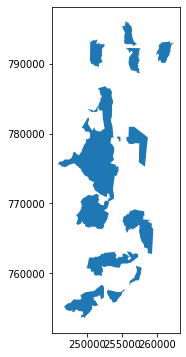
We can immediately see that the count Series contains values greater than 1 (up to 12), which means that there are towns represented by more than one row. For example, the regional council named "מבואות החרמון" is composed of 12 separate parts:
towns[towns['Muni_Heb'] == 'מבואות החרמון']
| Muni_Heb | Machoz | Shape_Area | geometry | area_km2 | |
|---|---|---|---|---|---|
| 88 | מבואות החרמון | צפון | 3.610206e+06 | POLYGON Z ((256646.431 792500.5... | 3.610206 |
| 89 | מבואות החרמון | צפון | 5.610637e+06 | POLYGON Z ((252583.953 792643.3... | 5.610637 |
| 90 | מבואות החרמון | צפון | 4.515282e+06 | POLYGON Z ((262438.235 792883.0... | 4.515282 |
| 91 | מבואות החרמון | צפון | 4.447152e+06 | POLYGON Z ((257523.972 791631.4... | 4.447152 |
| 92 | מבואות החרמון | צפון | 6.743527e+07 | POLYGON Z ((253621.386 770548.1... | 67.435270 |
| ... | ... | ... | ... | ... | ... |
| 95 | מבואות החרמון | צפון | 1.336877e+07 | POLYGON Z ((259270.552 762725.8... | 13.368774 |
| 96 | מבואות החרמון | צפון | 1.238126e+07 | POLYGON Z ((256798.730 762797.8... | 12.381256 |
| 97 | מבואות החרמון | צפון | 1.699528e+06 | POLYGON Z ((256108.896 758208.2... | 1.699528 |
| 98 | מבואות החרמון | צפון | 1.077375e+07 | POLYGON Z ((252450.242 756858.5... | 10.773754 |
| 99 | מבואות החרמון | צפון | 2.424360e+06 | POLYGON Z ((255326.620 757732.8... | 2.424360 |
12 rows × 5 columns
towns[towns['Muni_Heb'] == 'מבואות החרמון'].plot()
<AxesSubplot:>
We can also see that all geometries are of type "Polygon":
towns['geometry'].geom_type.value_counts()
Polygon    410
dtype: int64
We will see, in a moment that aggregation of a "Polygon" layer may create "MultiPolygon" geometries. For example, as a result of dissolving the towns layer by town name, the 12 rows with "Polygon" geometries of "מבואות החרמון" are going to turn into one row, with a "MultiPolygon" geometry (see below, Dissolving by town name).
Dissolving by town name#
Usually we want to have each towns’ information in a single row, to treat it as one unit. For instance, we usually are interested in the total .area of all parts of each town, at once, even if they are discontinuous in space. Therefore, we prefer to work with an aggregated the towns layer, grouping by town names ("Muni_Heb").
With geopandas, a vector layer can be aggregated using the .dissolve method, specifying:
by—The name of the column used for to groupingaggfunc—The function used to summarize the non-spatial columns:"first"(the default)"last""min""max""sum""mean""median"
For example, the following expression aggregates the towns layer by town name ("Muni_Heb"), taking the first value of all other attributes per town:
towns = towns.dissolve(by='Muni_Heb')
towns
| geometry | Machoz | Shape_Area | area_km2 | |
|---|---|---|---|---|
| Muni_Heb | ||||
| אבו גוש | POLYGON Z ((209066.649 635655.2... | ירושלים | 1.891242e+06 | 1.891242 |
| אבו סנאן | POLYGON Z ((212294.953 763168.8... | צפון | 6.455340e+06 | 6.455340 |
| אבן יהודה | POLYGON Z ((189803.359 684152.9... | מרכז | 8.141962e+06 | 8.141962 |
| אום אל פחם | MULTIPOLYGON Z (((212458.789 71... | חיפה | 2.988196e+05 | 0.298820 |
| אופקים | POLYGON Z ((164806.146 577898.8... | דרום | 1.635240e+07 | 16.352399 |
| ... | ... | ... | ... | ... |
| שפרעם | POLYGON Z ((215213.126 744570.3... | צפון | 1.962968e+07 | 19.629682 |
| תל אביב - יפו | POLYGON Z ((183893.870 668086.9... | תל אביב | 5.709679e+07 | 57.096785 |
| תל מונד | POLYGON Z ((190787.125 681015.0... | מרכז | 7.126864e+06 | 7.126864 |
| תל שבע | POLYGON Z ((186092.189 571779.8... | דרום | 9.421072e+06 | 9.421072 |
| תמר | MULTIPOLYGON Z (((207660.539 55... | דרום | 1.597418e+09 | 1597.417603 |
290 rows × 4 columns
Just like in ordinary aggregation, the column which is used for grouping is automatically transferred to the index of the resulting GeoDataFrame. To place it back to an ordinary column, we can use the .reset_index method (see Resetting the index):
towns = towns.reset_index()
towns
| Muni_Heb | geometry | Machoz | Shape_Area | area_km2 | |
|---|---|---|---|---|---|
| 0 | אבו גוש | POLYGON Z ((209066.649 635655.2... | ירושלים | 1.891242e+06 | 1.891242 |
| 1 | אבו סנאן | POLYGON Z ((212294.953 763168.8... | צפון | 6.455340e+06 | 6.455340 |
| 2 | אבן יהודה | POLYGON Z ((189803.359 684152.9... | מרכז | 8.141962e+06 | 8.141962 |
| 3 | אום אל פחם | MULTIPOLYGON Z (((212458.789 71... | חיפה | 2.988196e+05 | 0.298820 |
| 4 | אופקים | POLYGON Z ((164806.146 577898.8... | דרום | 1.635240e+07 | 16.352399 |
| ... | ... | ... | ... | ... | ... |
| 285 | שפרעם | POLYGON Z ((215213.126 744570.3... | צפון | 1.962968e+07 | 19.629682 |
| 286 | תל אביב - יפו | POLYGON Z ((183893.870 668086.9... | תל אביב | 5.709679e+07 | 57.096785 |
| 287 | תל מונד | POLYGON Z ((190787.125 681015.0... | מרכז | 7.126864e+06 | 7.126864 |
| 288 | תל שבע | POLYGON Z ((186092.189 571779.8... | דרום | 9.421072e+06 | 9.421072 |
| 289 | תמר | MULTIPOLYGON Z (((207660.539 55... | דרום | 1.597418e+09 | 1597.417603 |
290 rows × 5 columns
Note that we now have the same number of rows as the number of unique town names. Also note that some of the geometries are now of type "MultiPolygon" (why?):
towns['geometry'].geom_type.value_counts()
Polygon         228
MultiPolygon     62
dtype: int64
For example, here is the single entry for "מבואות החרמון", which is now a "MultiPolygon" (composed of 12 parts):
towns[towns['Muni_Heb'] == 'מבואות החרמון']
| Muni_Heb | geometry | Machoz | Shape_Area | area_km2 | |
|---|---|---|---|---|---|
| 182 | מבואות החרמון | MULTIPOLYGON Z (((252449.171 75... | צפון | 3.610206e+06 | 3.610206 |
Finally, the "Shape_Area" and "area_km2" columns are no longer correct (why?). We can drop one of them, and re-calculate the other:
towns = towns.drop('Shape_Area', axis=1)
towns['area_km2'] = towns.area / 1000**2
towns
| Muni_Heb | geometry | Machoz | area_km2 | |
|---|---|---|---|---|
| 0 | אבו גוש | POLYGON Z ((209066.649 635655.2... | ירושלים | 1.891242 |
| 1 | אבו סנאן | POLYGON Z ((212294.953 763168.8... | צפון | 6.455340 |
| 2 | אבן יהודה | POLYGON Z ((189803.359 684152.9... | מרכז | 8.141962 |
| 3 | אום אל פחם | MULTIPOLYGON Z (((212458.789 71... | חיפה | 26.028286 |
| 4 | אופקים | POLYGON Z ((164806.146 577898.8... | דרום | 16.352399 |
| ... | ... | ... | ... | ... |
| 285 | שפרעם | POLYGON Z ((215213.126 744570.3... | צפון | 19.629682 |
| 286 | תל אביב - יפו | POLYGON Z ((183893.870 668086.9... | תל אביב | 57.096785 |
| 287 | תל מונד | POLYGON Z ((190787.125 681015.0... | מרכז | 7.126864 |
| 288 | תל שבע | POLYGON Z ((186092.189 571779.8... | דרום | 9.421072 |
| 289 | תמר | MULTIPOLYGON Z (((207660.539 55... | דרום | 1623.029870 |
290 rows × 4 columns
Here is the revised entry for "מבואות החרמון":
towns[towns['Muni_Heb'] == 'מבואות החרמון']
| Muni_Heb | geometry | Machoz | area_km2 | |
|---|---|---|---|---|
| 182 | מבואות החרמון | MULTIPOLYGON Z (((252449.171 75... | צפון | 134.816362 |
Dissolving by district#
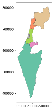
As another example of dissolving, let us now use "Machoz" (district) as the grouping column. This refers to a higher-level administrative division, and there are just six districts in Israel. The dissoved layer is thus composed of six features:
districts = towns.dissolve(by='Machoz').reset_index()
districts
| Machoz | geometry | Muni_Heb | area_km2 | |
|---|---|---|---|---|
| 0 | דרום | POLYGON Z ((214342.276 467536.8... | אופקים | 16.352399 |
| 1 | חיפה | MULTIPOLYGON Z (((205862.732 70... | אום אל פחם | 26.028286 |
| 2 | ירושלים | POLYGON Z ((192405.812 638419.6... | אבו גוש | 1.891242 |
| 3 | מרכז | MULTIPOLYGON Z (((171159.359 63... | אבן יהודה | 8.141962 |
| 4 | צפון | MULTIPOLYGON Z (((204805.266 71... | אבו סנאן | 6.455340 |
| 5 | תל אביב | POLYGON Z ((177312.943 655809.6... | אור יהודה | 6.730024 |
Here is a visualization of the resulting layer, colored by "Machoz" name so that we can see the placement of the regions in geographical space:
districts.plot(column='Machoz', cmap='Set2', edgecolor='black', linewidth=0.2);
Again, the "Muni_Heb" and "area_km2" attributes reflect the first value for each district and are no longer correct. We can either edit them manually (see Dissolving by town name), or use aggfunc other than 'first' (see below, Using aggfunc).
Using aggfunc#
As an example of using other aggfunc options, let us re-calculate the "Machoz" polygons, this time using aggfunc="sum". Note that the function is automatically applied on the relevant (i.e., numeric) columns, in this case the "Shape_Area" and "area" columns.
districts = towns.dissolve(by='Machoz', aggfunc='sum').reset_index()
districts
| Machoz | geometry | area_km2 | |
|---|---|---|---|
| 0 | דרום | POLYGON Z ((214342.276 467536.8... | 14476.526645 |
| 1 | חיפה | MULTIPOLYGON Z (((205862.732 70... | 895.010307 |
| 2 | ירושלים | POLYGON Z ((192405.812 638419.6... | 653.586307 |
| 3 | מרכז | MULTIPOLYGON Z (((171159.359 63... | 1312.566854 |
| 4 | צפון | MULTIPOLYGON Z (((204805.266 71... | 4649.160352 |
| 5 | תל אביב | POLYGON Z ((177312.943 655809.6... | 179.168299 |
This time, in the dissolved result, the "area" column contains the summed area of all geometries in each group, which is the correct value. Compare with the above result, where the column contained the value of just the first geometry, which is incorrect.
Geometric relations#
The geopandas package contains a series of functions to evaluate spatial relations between geometries. For instance, in the next example, we are interested to examine which railway stations intersect with the area of Beer-Sheva, and then to subset those stations. To do that, in technical terms, we need to evaluate whether each geometry in the stations layer intersects with a particular geometry (Beer-Sheva) in the towns layer.
The geopandas package defines functions of the same name, analogous to the shapely boolean functions (see shapely boolean methods). Of those, .intersects is the most useful one. While the shapely version of .intersects returns a single boolean value, indicating whether the two geometries intersect (see Boolean functions), the geopandas version returns a boolean Series with pairwise results. There are two modes of operation:
Pairwise results between two
GeoSeriesaligned by index or by positionResults between all geometries in a
GeoSeriesand a singleshapelygeometry
In this example, we are going to demonstrate the second (simpler) workflow of .intersects, where we have a GeoSeries or a GeoDataFrame on the one hand, and an individual shapely geometry on the other hand.
First of all, let us subset the towns layer to retain just the Beer-Sheva shapely polygon, as follows:
pol = towns[towns['Muni_Heb'] == 'באר שבע']
pol
| Muni_Heb | geometry | Machoz | area_km2 | |
|---|---|---|---|---|
| 22 | באר שבע | POLYGON Z ((175342.311 568405.3... | דרום | 117.393493 |
Here a visualization of the individual geometry from pol:
pol['geometry'].iloc[0]

Now, we are ready to evaluate the intersection between stations, on the one hand, and the pol geometry, on the other hand, using the .intersects method:
sel = stations.intersects(pol['geometry'].iloc[0])
sel
0     False
1     False
2     False
3     False
4     False
      ...
58    False
59     True
60    False
61    False
62    False
Length: 63, dtype: bool
The result sel is a boolean Series, indicating for each stations feature whether it intersects with the Beer-Sheva polygon.
Exercise 09-e
How can we check how many of the
stationsfeatures intersect with the polygon, i.e., to count the number ofTruevalues in theselseries?
Using the boolean Series from the previous code section, we can subset (see DataFrame filtering) the railway stations that are within Beer-Sheva:
stations[sel]
| STAT_NAMEH | ON_7_DAY | OFF_7_DAY | ON_17_DAY | OFF_17_DAY | geometry | nearest_seg_dist | nearest_seg_name | |
|---|---|---|---|---|---|---|---|---|
| 41 | באר שבע מרכז | 0.0 | 174.0 | 0.0 | 181.0 | POINT (180768.910 572476.735) | 34.113422 | באר שבע אוניברסיטה - באר שבע |
| 59 | באר שבע אוניברסיטה | 212.0 | 130.0 | 89.0 | 184.0 | POINT (181813.614 574550.411) | 7.540327 | באר שבע צפון - באר שבע אוניב |
Here is the plot of the resulting stations subset, on top of the town polygon used for filtering them:
base = pol.plot(color='none', edgecolor='grey')
stations[sel].plot(ax=base);
Note
The .intersects method has other, more complicated, modes of operation, such as examining pairwise relations between geometries from two GeoSeries (composed of more than one geometry). See the documentation for details: https://geopandas.readthedocs.io/en/latest/docs/reference/api/geopandas.GeoSeries.intersects.html. There are also analogous functions to evaluate standard spatial relations other than intersection, such as .crosses, .contains, .touches, .disjoint, etc.
Spatial join#
Ordinary spatial join#
Spatial join merges two spatial layers, in the same sense that an ordinary (i.e., non-spatial) join merges two tables (see Joining tables). The difference is that the features (i.e., rows) to join are not determined based on matching values in a common column. Instead, they are determined based on spatial relations. Typically, spatial join is based on the intersection (see Geometric relations), which means that we are joining attributes of feature(s) from the second layer, that intersect with the given feature in the first layer.
In geopandas, spatial join is done using the gpd.sjoin (“spatial join”) function. The gpd.sjoin function takes the following arguments:
The first (“left”) layer
The second (“right”) layer
how—The type of join, one of:'inner'(the default)'left''right'
predicate—The spatial relation to evaluate when looking for a match, one of:'intersects'(the default)'contains''crosses''overlaps''touches''within'
You may notice similarities with the pd.merge function for ordinary (non-spatial) join (see Joining tables). Namely, three of the four parameters are the same: the two tables/layers, and the how argument for join type. The difference is just the method for evaluating the matching rows/features:
In an ordinary join, matching rows are determined based on identical values in a common column, specified using the
onargument inpd.mergeIn a spatial join, matching features are determined based on spatial relations, such as whether the two features intersect or not, whereas the type of relation is specified using the
predicateargument ingpd.sjoin
For example, the following spatial join operation reveals, for each railway station, which town it intersects with (i.e., located within). We also limit the input layers to just one attribute each, to see more clearly what is going on:
gpd.sjoin(
    stations[['STAT_NAMEH', 'geometry']],
    towns[['Muni_Heb', 'geometry']],
    how='left'
)
| STAT_NAMEH | geometry | index_right | Muni_Heb | |
|---|---|---|---|---|
| 0 | ראשון לציון משה דיין | POINT (177206.094 655059.936) | 263 | ראשון לציון |
| 1 | קרית ספיר נתניה | POINT (187592.123 687587.598) | 219 | נתניה |
| 2 | ת"א השלום | POINT (180621.940 664537.210) | 286 | תל אביב - יפו |
| 3 | שדרות | POINT (160722.849 602798.889) | 283 | שער הנגב |
| 4 | רמלה | POINT (188508.910 648466.870) | 269 | רמלה |
| ... | ... | ... | ... | ... |
| 58 | מגדל העמק כפר ברוך | POINT (219851.931 728164.825) | 233 | עמק יזרעאל |
| 59 | באר שבע אוניברסיטה | POINT (181813.614 574550.411) | 22 | באר שבע |
| 60 | חיפה בת גלים | POINT (198610.010 748443.790) | 81 | חיפה |
| 61 | לוד | POINT (188315.977 650289.373) | 123 | לוד |
| 62 | נהריה | POINT (209570.590 767769.220) | 210 | נהריה |
63 rows × 4 columns
The spatial join result contains the attributes and geometry of the left layer, plus joined attributes and indices ("index_right") of the right layer. In this case, we have:
the
"STAT_NAMEH","geometry"columns from the “left”stationslayer, andthe
"index_right"and"Muni_Eng"columns joined from the “right”townslayer.
For example, the first feature in the spatial join result reveals that the "ראשון לציון משה דיין" station is located in the town "ראשון לציון".
As another, more complicated, example, the following spatial join might be a first attempt to can check which railway lines goes through each railway station:
gpd.sjoin(
    stations[['STAT_NAMEH', 'geometry']],
    rail,
    how='left'
)
| STAT_NAMEH | geometry | index_right | SEGMENT | length_km | |
|---|---|---|---|---|---|
| 0 | ראשון לציון משה דיין | POINT (177206.094 655059.936) | NaN | NaN | NaN |
| 1 | קרית ספיר נתניה | POINT (187592.123 687587.598) | NaN | NaN | NaN |
| 2 | ת"א השלום | POINT (180621.940 664537.210) | NaN | NaN | NaN |
| 3 | שדרות | POINT (160722.849 602798.889) | NaN | NaN | NaN |
| 4 | רמלה | POINT (188508.910 648466.870) | NaN | NaN | NaN |
| ... | ... | ... | ... | ... | ... |
| 58 | מגדל העמק כפר ברוך | POINT (219851.931 728164.825) | NaN | NaN | NaN |
| 59 | באר שבע אוניברסיטה | POINT (181813.614 574550.411) | NaN | NaN | NaN |
| 60 | חיפה בת גלים | POINT (198610.010 748443.790) | NaN | NaN | NaN |
| 61 | לוד | POINT (188315.977 650289.373) | NaN | NaN | NaN |
| 62 | נהריה | POINT (209570.590 767769.220) | NaN | NaN | NaN |
63 rows × 5 columns
In this case, we see that none, or at least the first and last few, stations, had a match. This means that none of the lines precisely intersect with the station points.
One way to overcome this is to use nearest-neighbor join (see Nearest neighbor join). Another option is to use a buffered version of the stations, say with a 100 \(m\) buffer. In this case, we join the attributes of the segments that are within a 100 \(m\) distance from each station:
stations1 = stations.copy()
stations1['geometry'] = stations1.buffer(100)
stations1[['STAT_NAMEH', 'geometry']]
| STAT_NAMEH | geometry | |
|---|---|---|
| 0 | ראשון לציון משה דיין | POLYGON ((177306.094 655059.936... |
| 1 | קרית ספיר נתניה | POLYGON ((187692.123 687587.598... |
| 2 | ת"א השלום | POLYGON ((180721.940 664537.210... |
| 3 | שדרות | POLYGON ((160822.849 602798.889... |
| 4 | רמלה | POLYGON ((188608.910 648466.870... |
| ... | ... | ... |
| 58 | מגדל העמק כפר ברוך | POLYGON ((219951.931 728164.825... |
| 59 | באר שבע אוניברסיטה | POLYGON ((181913.614 574550.411... |
| 60 | חיפה בת גלים | POLYGON ((198710.010 748443.790... |
| 61 | לוד | POLYGON ((188415.977 650289.373... |
| 62 | נהריה | POLYGON ((209670.590 767769.220... |
63 rows × 2 columns
Then, we join the buffered stations1 with the rail layer:
gpd.sjoin(
    stations1[['STAT_NAMEH', 'geometry']],
    rail,
    how='left'
)
| STAT_NAMEH | geometry | index_right | SEGMENT | length_km | |
|---|---|---|---|---|---|
| 0 | ראשון לציון משה דיין | POLYGON ((177306.094 655059.936... | 81.0 | משה דיין-חולות_82 | 1.851570 |
| 0 | ראשון לציון משה דיין | POLYGON ((177306.094 655059.936... | 22.0 | משה דיין-קוממיות_23 | 1.477394 |
| 1 | קרית ספיר נתניה | POLYGON ((187692.123 687587.598... | 100.0 | נתניה מכללה - נתניה ספיר_101 | 1.417325 |
| 2 | ת"א השלום | POLYGON ((180721.940 664537.210... | 79.0 | יצחק שדה - השלום_80 | 1.009135 |
| 2 | ת"א השלום | POLYGON ((180721.940 664537.210... | 57.0 | סבידור מרכז - השלום_58 | 1.286116 |
| ... | ... | ... | ... | ... | ... |
| 60 | חיפה בת גלים | POLYGON ((198710.010 748443.790... | 153.0 | חוף כרמל - בת גלים_156 | 6.121700 |
| 60 | חיפה בת גלים | POLYGON ((198710.010 748443.790... | 193.0 | השמונה - בת גלים_197 | 1.644544 |
| 61 | לוד | POLYGON ((188415.977 650289.373... | 77.0 | לוד - רמלה_78 | 1.339807 |
| 61 | לוד | POLYGON ((188415.977 650289.373... | 198.0 | לוד-רמלה מערב_203 | 1.412130 |
| 62 | נהריה | POLYGON ((209670.590 767769.220... | NaN | NaN | NaN |
113 rows × 5 columns
In this case, there are even stations with more than one matching line (e.g., "ראשון לציון משה דיין"), because there can be more than one railway segment passing through a radius of 100 \(m\) of a railway station. However, other stations still had zero matches (e.g., "נהריה"). This leads us to the second option of dealing with the situation, the nearest neighbor join (see below, Nearest neighbor join).
Exercise 09-f
Note that the last station (
"נהריה") has “No Data” in the segment name column ("SEGMENT"). Can you explain why?
Nearest neighbor join#
In addition to spatial join based on “ordinary” relations such as intersection (see Ordinary spatial join), the geopandas package also has a gpd.sjoin_nearest function for spatial join based on nearest neighbors. It works similarly to gpd.sjoin, but matches are determined based on shortest pairwise distance.
The following expression joins the nearest railway line attributes (including segment name, "SEGMENT") and specifies the distances in the "dist" column as requested using the distance_col="dist" argument:
stations = gpd.sjoin_nearest(
    stations[['STAT_NAMEH', 'nearest_seg_dist', 'nearest_seg_name', 'geometry']],
    rail[['SEGMENT', 'geometry']],
    distance_col='dist'
)
stations
| STAT_NAMEH | nearest_seg_dist | nearest_seg_name | geometry | index_right | SEGMENT | dist | |
|---|---|---|---|---|---|---|---|
| 0 | ראשון לציון משה דיין | 13.440327 | משה דיין-קוממיות_23 | POINT (177206.094 655059.936) | 22 | משה דיין-קוממיות_23 | 13.440327 |
| 12 | בת ים קוממיות | 2.711357 | משה דיין-קוממיות_23 | POINT (177404.549 656501.262) | 22 | משה דיין-קוממיות_23 | 2.711357 |
| 1 | קרית ספיר נתניה | 4.932094 | נתניה מכללה - נתניה ספיר_101 | POINT (187592.123 687587.598) | 100 | נתניה מכללה - נתניה ספיר_101 | 4.932094 |
| 2 | ת"א השלום | 16.180832 | סבידור מרכז - השלום_58 | POINT (180621.940 664537.210) | 57 | סבידור מרכז - השלום_58 | 16.180832 |
| 3 | שדרות | 64.381044 | שדרות-יד מרדכי_134 | POINT (160722.849 602798.889) | 131 | שדרות-יד מרדכי_134 | 64.381044 |
| ... | ... | ... | ... | ... | ... | ... | ... |
| 58 | מגדל העמק כפר ברוך | 56.102377 | עפולה - כפר ברוך_155 | POINT (219851.931 728164.825) | 152 | עפולה - כפר ברוך_155 | 56.102377 |
| 59 | באר שבע אוניברסיטה | 7.540327 | באר שבע צפון - באר שבע אוניב | POINT (181813.614 574550.411) | 205 | באר שבע צפון - באר שבע אוניב | 7.540327 |
| 60 | חיפה בת גלים | 44.130049 | חוף כרמל - בת גלים_156 | POINT (198610.010 748443.790) | 153 | חוף כרמל - בת גלים_156 | 44.130049 |
| 61 | לוד | 22.556829 | לוד - רמלה_78 | POINT (188315.977 650289.373) | 77 | לוד - רמלה_78 | 22.556829 |
| 62 | נהריה | 115.502833 | נהריה - עכו_13 | POINT (209570.590 767769.220) | 12 | נהריה - עכו_13 | 115.502833 |
63 rows × 7 columns
This time, we get exactly one matching rail segment per stations point. In addition to the segment name ("SEGMENT"), the distance to the matched nearest segment is documented in the "dist" column. As you can see, the values in these two columns are identical to the "nearest_seg_name" and "nearest_seg_dist" columns, respectively, which we calculated earlier using a “manual” approach (see Nearest neighbors):
(stations['nearest_seg_name'] == stations['SEGMENT']).all()
True
(stations['nearest_seg_dist'] == stations['dist']).all()
True
Note
For more information, see the gpd.sjoin_nearest function documentation: https://geopandas.org/en/stable/docs/reference/api/geopandas.sjoin_nearest.html.
More exercises#
Exercise 09-g
Read the towns (
muni_il.shp) layers (see Sample data)Aggregate it according to the
"Machoz"column to dissolve the towns into district polygons (see Dissolving by district)Calculate the number of neighbors, i.e., districts it intersects with excluding self, that each district has.
Plot the result (Fig. 56).
Advanced: display labels with the number of neighbors per district (Fig. 56), by adapting this StackOverflow answer.
Hint:
Aggregate the towns layer according to the
"Machoz"column to dissolve the towns into district polygons (see Aggregation (.dissolve)).Join the layer with itself, based on “intersection”, to join each town with all of its neighbors, then use aggregation to calculate the sum of joined towns per town. You can create a
"count"variable for each town, equal to1, then sum it when calculating the number of neighbors.Subtract
1to get the number of intersections excluding intersection with self, i.e., the number of neighbors.
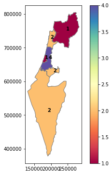
Fig. 56 Solution of exercise-09-g: Neighbor count per town#
Exercise 09-h
Calculate the total population size in a 1 \(km\) buffer around each railway station in
RAIL_STAT_ONOFF_MONTH.shp, according to the population data instatisticalareas_demography2019.gdb(Pop_Total=total population).Sort the table, to see which stations are situated in the most dense and sparse areas (Fig. 57).
Go through the following steps:
Import both layers into
GeoDataFrameobjects.Calculate the area of each statistical area polygon.
Fill the missing population estimates (in the
Pop_Totalcolumn) with zeros.Create a buffer of 1 \(km\) around the station points.
Calculate a layer of pairwise intersections between the buffers and the statistical areas.
Calculate the area of each intersection.
Calculate the population count of each intersection. To do that, multiply the statistical area population count column (
Pop_Total) by the ratio between the intersection area, and the original total area of that statistical area (which you calculated in the second step earlier).Aggregate the layer by rail station name, to calculate the total population count per 1 \(km\) buffer around a station.
Sort the layer by population counts, to see which stations are situated in the most dense and sparse areas.
| geometry | pop1 | |
|---|---|---|
| name | ||
| בת ים יוספטל | POLYGON ((177152.750 657153.746, 177103.606 65... | 55761.058635 |
| ירושלים יצחק נבון | POLYGON ((218650.757 632087.423, 218578.044 63... | 46441.448009 |
| ת"א סבידור מרכז | POLYGON ((180306.847 665089.717, 180277.411 66... | 39493.940946 |
| חולון וולפסון | POLYGON ((176806.558 659551.427, 176733.844 65... | 35295.776253 |
| קרית מוצקין | POLYGON ((206654.795 747716.120, 206559.600 74... | 35148.940155 |
| ... | ... | ... |
| מגדל העמק כפר ברוך | POLYGON ((218894.991 727874.541, 218871.146 72... | 29.732200 |
| קרית מלאכי יואב | POLYGON ((184266.430 628244.915, 184252.031 62... | 0.000000 |
| חוצות המפרץ | POLYGON ((205604.630 745103.145, 205507.557 74... | 0.000000 |
| פאתי מודיעין | POLYGON ((197394.885 644447.483, 197380.485 64... | 0.000000 |
| יקנעם כפר יהושוע | POLYGON ((212300.180 731084.998, 212211.467 73... | 0.000000 |
63 rows × 2 columns
Fig. 57 Solution of exercise-09-h: Railway stations with largest and smallest population counts in a 1 km buffer#
Exercise 09-i
Read the following vector layers (see Sample data):
Towns (
muni_il.shp)Railway lines (
RAIL_STRATEGIC.shp)
Aggregate the towns layer according to the
"Muni_Heb"column to dissolve the separate polygons per town (see Aggregation (.dissolve)).Subset only the active railway lines, i.e., where the value in the
"ISACTIVE"column is equal to"פעיל"(see Filtering by attributes).Subset the town polygons that a railway line goes through.
Plot the resulting subset of towns and the active railway lines together (Fig. 58).
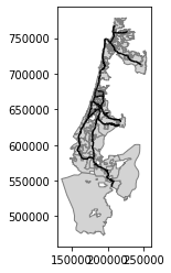
Fig. 58 Solution of exercise-09-i: Towns (grey polygons) intersecting with active railway lines (black lines)#