Tables (`pandas`)#

Last updated: 2023-02-25 13:41:46

Introduction#

Tables are a fundamental data structure, common to many software interfaces, such as spreadsheet programs, relational databases, statistical software, etc. In general, a table is a two-dimensional structure where:

Columns represent variables
Rows represent observations

Accordingly, the data in a given table column is usually of the same data type. For example, a text column may be used to store product names, and a numeric column may be used for storing product prices. Conversely, the data in a given row may comprise mixed types, such as the product name (text) and the price (numeric) of a particular product.

In this chapter we introduce methods for working with tables in Python, through a popular third-party package named pandas, introducing two table-related data structures, Series and DataFrame. As we will see, the latter data structures are closely related to numpy, which was covered in the previous chapter (see Arrays (numpy)), since the data in each table column is actually stored as an “extended” one-dimensional numpy array. We are going to cover standard table-related operations, such as:

Creating tables (see Creating from scratch and Reading from file)
Examining table properties (see DataFrame properties)
Modifying tables (see Renaming columns, Modifying the index, Sorting, Operators, and Creating new columns)
Subsetting tables (see Subsetting Series, Subsetting DataFrames, and DataFrame filtering)
Working with missing data (pandas)
Conversion to simpler data structures (see Convertsion to ndarray and Conversion to list)
Plotting table data (see Plotting (pandas))
Exporting a table to file (see Writing to file)

In the next chapter, we are going to discuss more advanced operations with tables, such as table aggregation and table joins (see Table reshaping and joins). Later on, we are going to learn about the geopandas package for working with vector layers, which is an extension of pandas (see Vector layers (geopandas) and Geometric operations).

What is `pandas`?#

pandas is a popular Python package which provides a flexible set of tools for working with tabular data. Since tables are fundamental in data analysis, pandas is one of the most important packages for data analysis in Python. Moreover, as we will see later on in the book (see Vector layers (geopandas)), a vector layers is represented by an “extended” table—a table that has a “geometry” column. Accordingly, the package for working with vector later, named geopandas, is an extension of pandas.

The pandas package defines two fundamental data structures:

Series—A one-dimensional structure, representing a table column
DataFrame—A two-dimensional structure, represent a table

As we will see shortly, pandas is essentially an extension of numpy. A pandas table (a data structure named DataFrame) is a collection of Series representing the table columns, whereas Series are actually nothing more than labelled numpy arrays. To repeat, these two data structures therefore form a hierarchy: each column in a DataFrame is a Series.

Note

For those familiar with the R programming language, the term DataFrame will sound familiar, resembling R’s own data structure for representing tables (the data.frame). Indeed, pandas borrowed many ideas from the R language. A pairwise comparison of pandas vs. R functionality can be found in the pandas documentation: https://pandas.pydata.org/docs/getting_started/comparison/comparison_with_r.html

Creating from scratch#

Creating a `Series`#

To understand how a DataFrame is structured, we will experiment with creating one from scratch. First we need to load the pandas package, as well as numpy which we use in some of the examples:

import numpy as np
import pandas as pd

A Series can be created, from a list, or from an ndarray, using pd.Series. For example, the following expression creates a Series from a list containing three strings, the names of three railway stations in southern Israel:

name = pd.Series(['Beer-Sheva Center', 'Beer-Sheva University', 'Dimona'])
name

      Beer-Sheva Center
  Beer-Sheva University
                 Dimona
dtype: object

Note

In pandas, strings are always stored as 'object' arrays (Series), unlike numpy which has specialized native data types for strings.

The following expression creates another Series, named lines, containing the number of railway lines going through the latter stations. This time, we create the Series from an ndarray:

lines = pd.Series(np.array([4, 5, 1]))
lines

  4
  5
  1
dtype: int64

A Series object is essentially a numpy array, combined with indices. Here is how we can access each of these components, separately:

lines.to_numpy()  ## Series values, as 'ndarray'

array([4, 5, 1])

lines.index       ## Series index

RangeIndex(start=0, stop=3, step=1)

As you can see, Series values comprise a numpy array, which we are already familiar with. Series indices, however, comprise a special type of object used for indexing in pandas:

type(name.index)

pandas.core.indexes.range.RangeIndex

By default, the index is just a sequence of consecutive integers (such as in names and lines). When necessary, we can define any other sequence of values as a Series index (see Modifying the index), then use it to access specific values (see Subsetting Series).

Index objects are similar to arrays in many ways. For example, they have .shape and .dtype attributes, just like arrays do:

lines.index.shape

(3,)

lines.index.dtype

dtype('int64')

Creating a `DataFrame`#

While a Series can be thought of as an extended one-dimensional array, a DataFrame can be thought of as a collection of Series comprising table columns. Unlike a two-dimensional numpy array, a DataFrame can be composed of different types of values (among the columns). Consequently:

a DataFrame column (i.e., a Series) contains values of the same type, usually representing a particular variable
a DataFrame row may contain values of different types, usually representing a specific observation

Since a DataFrame is two-dimensional, it has two sets of idices, row and column indices, just like a two-dimensional array. It is important to note that all Series that comprise the columns of a DataFrame share the same index.

A DataFrame can be created from scratch, using the pd.DataFrame function. To do that, let us create four more Series which are going to comprise the DataFrame columns. Altogether, the DataFrame is going to represent various properties of three railway stations:

city = pd.Series(['Beer-Sheva', 'Beer-Sheva', 'Dimona'])
piano = pd.Series([False, True, False])
lon = pd.Series([34.798443, 34.812831, 35.011635])
lat = pd.Series([31.243288, 31.260284, 31.068616])

Here is a printout of the four Series we just created:

city

  Beer-Sheva
  Beer-Sheva
      Dimona
dtype: object

piano

  False
   True
  False
dtype: bool

lon

  34.798443
  34.812831
  35.011635
dtype: float64

lat

  31.243288
  31.260284
  31.068616
dtype: float64

Now, the six different Series can be combined into a DataFrame by passing them, as a dict (see Dictionaries (dict)), to the pd.DataFrame function. That way, the dict names will form the DataFrame column names, while the corresponding Series will form the column contents:

d = {'name': name, 'city': city, 'lines': lines, 'piano': piano, 'lon': lon, 'lat': lat}
stations = pd.DataFrame(d)
stations

	name	city	lines	piano	lon	lat
0	Beer-Sheva Center	Beer-Sheva	4	False	34.798443	31.243288
1	Beer-Sheva University	Beer-Sheva	5	True	34.812831	31.260284
2	Dimona	Dimona	1	False	35.011635	31.068616

Note

Note that there are other methods to create a DataFrame, passing different types of input to the pd.DataFrame function. For example, another useful method of creating a DataFrame by passing a two-dimensional array to pd.DataFrame.

DataFrame row indices are analogous to Series indices, and accessed exactly the same way:

stations.index

RangeIndex(start=0, stop=3, step=1)

Additionally, a DataFrame has column indices, which function as column names and can be accessed through the .columns property:

stations.columns

Index(['name', 'city', 'lines', 'piano', 'lon', 'lat'], dtype='object')

Reading from file#

In practice, we rarely need to create a DataFrame from scratch. More often, we read a table in an existing file containing tabular data, such as a CSV file.

The pd.read_csv function is used to read a CSV file into a DataFrame in our Python environment. For example, the following expression reads the CSV file named ZonAnn.Ts+dSST.csv, which contains global temperature data from GISS. The values are anomalies, i.e. deviations from the corresponding 1951-1980 mean, for the period 1880-2021 ("Year"), both globally ("Glob") and for specific latitudes ("NHem"=Nothern Hemishpere, "24N-90N" latitudes 24-90, etc.):

dat = pd.read_csv('data/ZonAnn.Ts+dSST.csv')
dat

	Year	Glob	NHem	SHem	24N-90N	...	EQU-24N	24S-EQU	44S-24S	64S-44S	90S-64S
0	1880	-0.16	-0.29	-0.04	-0.37	...	-0.15	-0.09	-0.03	0.05	0.65
1	1881	-0.08	-0.17	0.01	-0.34	...	0.10	0.12	-0.05	-0.07	0.57
2	1882	-0.11	-0.21	0.00	-0.31	...	-0.05	-0.04	0.02	0.04	0.60
3	1883	-0.17	-0.28	-0.06	-0.35	...	-0.17	-0.14	-0.03	0.07	0.48
4	1884	-0.28	-0.43	-0.14	-0.61	...	-0.13	-0.15	-0.19	-0.02	0.63
...	...	...	...	...	...	...	...	...	...	...	...
137	2017	0.92	1.18	0.67	1.40	...	0.87	0.77	0.76	0.35	0.55
138	2018	0.85	1.04	0.66	1.25	...	0.73	0.62	0.79	0.37	0.96
139	2019	0.98	1.22	0.75	1.43	...	0.91	0.89	0.74	0.39	0.83
140	2020	1.02	1.36	0.68	1.68	...	0.89	0.84	0.58	0.39	0.91
141	2021	0.85	1.15	0.55	1.43	...	0.73	0.59	0.71	0.32	0.33

142 rows × 15 columns

Note

pandas has several functions named pd.read_* to read formats other than CSV, such as pd.read_json, pd.read_excel, pd.read_spss, pd.read_stata, and pd.read_sql. Similarly, there are several functions to write DataFrame objects to various output formats. See the IO tools section in the pandas user guide for an overview of the input/output capabilities.

Note that rows and columns are labelled using indices, as shown above. In this case:

Rows are labelled with consecutive integers
Columns are labelled with column names, which are imported from the first line in CSV file

`DataFrame` properties#

Overview#

One of the first things we may want to do with a DataFrame imported from a file is to examine its properties, as shown in the next few sections:

DataFrame dimensions
DataFrame column names
DataFrame column types

`DataFrame` dimensions#

DataFrame dimensions are accessible through the .shape property, just like in a numpy array (see Array dimensions). For example, the dat table (with the temperature data) has 142 rows and 15 columns:

dat.shape

(142, 15)

`DataFrame` column names#

The DataFrame column names can be obtained through the .columns property. Recall that this is a special data structure representing pandas indices (see Creating from scratch):

dat.columns

Index(['Year', 'Glob', 'NHem', 'SHem', '24N-90N', '24S-24N', '90S-24S',
       '64N-90N', '44N-64N', '24N-44N', 'EQU-24N', '24S-EQU', '44S-24S',
       '64S-44S', '90S-64S'],
      dtype='object')

Exercise 05-a

From your experience with Python so far, can you guess how can the columns names be transformed to a plain list? (You can also try searching for the answer online.)

`DataFrame` column types#

The data types (see Data types) of the columns are contained in the dtypes property:

dat.dtypes

Year         int64
Glob       float64
NHem       float64
SHem       float64
24N-90N    float64
            ...   
EQU-24N    float64
24S-EQU    float64
44S-24S    float64
64S-44S    float64
90S-64S    float64
Length: 15, dtype: object

Note that this is a Series (of dtype objects). This means we can get a specific value by index using the ordinary Series subsetting methods which we learn about later on (see Subsetting Series). For example, the "Year" column was imported into a Series of type int64:

dat.dtypes.loc['Year']

dtype('int64')

while the "Glob" column (global temperature anomaly) was imported into a float64 column:

dat.dtypes.loc['Glob']

dtype('float64')

The basic pandas data types are in agreement with numpy data types (see Data types). For example, the dat table contains int64 and float64 data types. However, pandas and its extensions (such as geopandas, see What is geopandas?) also extend the numpy functionality with new data types (such as GeometryDtype, see GeoSeries (geometry) column).

Renaming columns#

Sometimes it is necessary to rename DataFrame columns. For example, we may wish to use shorter names which are easier to type, or make the columns match another table we are working with. Columns can be renamed using the .rename method, which accepts a columns argument of the form {'old_name':'new_name',...}. For example, here is how we can replace the 'Year' column name with lowercase 'year':

dat.rename(columns={'Year': 'year'})

	year	Glob	NHem	SHem	24N-90N	...	EQU-24N	24S-EQU	44S-24S	64S-44S	90S-64S
0	1880	-0.16	-0.29	-0.04	-0.37	...	-0.15	-0.09	-0.03	0.05	0.65
1	1881	-0.08	-0.17	0.01	-0.34	...	0.10	0.12	-0.05	-0.07	0.57
2	1882	-0.11	-0.21	0.00	-0.31	...	-0.05	-0.04	0.02	0.04	0.60
3	1883	-0.17	-0.28	-0.06	-0.35	...	-0.17	-0.14	-0.03	0.07	0.48
4	1884	-0.28	-0.43	-0.14	-0.61	...	-0.13	-0.15	-0.19	-0.02	0.63
...	...	...	...	...	...	...	...	...	...	...	...
137	2017	0.92	1.18	0.67	1.40	...	0.87	0.77	0.76	0.35	0.55
138	2018	0.85	1.04	0.66	1.25	...	0.73	0.62	0.79	0.37	0.96
139	2019	0.98	1.22	0.75	1.43	...	0.91	0.89	0.74	0.39	0.83
140	2020	1.02	1.36	0.68	1.68	...	0.89	0.84	0.58	0.39	0.91
141	2021	0.85	1.15	0.55	1.43	...	0.73	0.59	0.71	0.32	0.33

142 rows × 15 columns

Note

Another option to rename columns is to assign a list of strings of the same length as the number of columns to the .columns attribute (see https://stackoverflow.com/questions/11346283/renaming-column-names-in-pandas#answer-11346337).

Subsetting in `pandas`#

There are numerous methods of subsetting Series and DataFrames in pandas. For example, Series values can be subsetted using the [ operator. However, this can be confusing since both using numeric indices and the index values are permitted, and it can be unclear which method is actually employed.

In agreement with the Python philosophy, where explicit is better than implicit, the recommended subsetting methods are using .loc and .iloc, which are discussed in the following sub-sections. The principal difference between .loc and .iloc is:

.loc uses pandas indices, while
.iloc uses (implicit) numpy-style numeric indices.

In this book, we are going to use .iloc and .loc methods when subsetting Series (this section) and DataFrame (see Subsetting DataFrames) objects. Nevertheless, for shorter syntax, in three exceptions we are going to use the [ shortcut as follows:

Selecting DataFrame columns using the [ operator, as in:
- dat['Year'] instead of dat.loc[:,'Year'] (see Selecting DataFrame columns)
- dat[['Year']] instead of dat.loc[:,['Year']] (see Selecting DataFrame columns)
Filtering DataFrame rows using the [ operator, as in:
- dat[dat['Year']>2017] instead of dat.loc[dat['Year']>2017] (see DataFrame filtering)

Subsetting `Series`#

As mentioned above, the recommended way to subset Series is using the specialized methods named .loc and .iloc:

.loc—For subsetting using the Series index
.iloc—For subsetting using the (implicit) numpy index

What follows after the method are the indices, inside square brackets ([), whereas the indices can be one of:

An individual value, such as .loc['a'] or .iloc[0]
A slice, such as .loc['a':'b'] or .iloc[1:2]
A list, such as .loc[['a','c']] or .iloc[[0,2]]

For the next few examples, let us create a Series object named s, with:

values 11, 12, 13, 14, and
indices 'a', 'b', 'c', 'd',

using the index parameter of pd.Series:

s = pd.Series([11, 12, 13, 14], index=['a', 'b', 'c', 'd'])
s

a    11
b    12
c    13
d    14
dtype: int64

Here is how we can use .loc to select values using the three above-mentioned types of indices:

s.loc['a']         ## Individual index

s.loc['b':'c']     ## Slice

b    12
c    13
dtype: int64

s.loc[['a', 'c']]  ## 'list' of indices

a    11
c    13
dtype: int64

And here is how we can use .iloc to select values using numpy-style numeric indices:

s.iloc[0]       ## Individual index

s.iloc[1:2]     ## Slice

b    12
dtype: int64

s.iloc[[0, 2]]  ## 'list' of indices

a    11
c    13
dtype: int64

In the above examples, note how using an individual index returns a standalone value, while using a slice, or a list of indices, return a Series, even if the list or the slice contains just one element:

s.iloc[[0]]

a    11
dtype: int64

Also note that a slice using indices (such as s.loc["a":"b"]) is inclusive, while a slice using implicit indices (such as .iloc[0:1]) excludes the last index similarly to list and numpy behavior.

Subsetting `DataFrame`s#

Selecting `DataFrame` columns#

A DataFrame is a two-dimensional object, unlike a Series which is one-dimensional. Accordingly, the .loc and iloc methods of a DataFrame accept two indices, separated by a comma:

The first index refers to rows
The second index refers to columns

When we want to select all rows or columns, we place : in the respective index, similarly to numpy array subsetting (see Subsetting arrays). Using an individual index returns a Series, while using a slice or a list of indices—even if length 1—returns a DataFrame.

For example, this is how we can use .loc to extract one DataFrame column as a Series:

dat.loc[:, 'Glob']

   -0.16
   -0.08
   -0.11
   -0.17
   -0.28
       ... 
  0.92
  0.85
  0.98
  1.02
  0.85
Name: Glob, Length: 142, dtype: float64

and here is how we can extract a single column as a DataFrame:

dat.loc[:, ['Glob']]

	Glob
0	-0.16
1	-0.08
2	-0.11
3	-0.17
4	-0.28
...	...
137	0.92
138	0.85
139	0.98
140	1.02
141	0.85

142 rows × 1 columns

As mentioned above (see Subsetting in pandas), we can also use the shortcut [ operator to subset columns(s):

dat['Glob']  ## Shortcut for `dat.loc[:, 'Glob']`

   -0.16
   -0.08
   -0.11
   -0.17
   -0.28
       ... 
  0.92
  0.85
  0.98
  1.02
  0.85
Name: Glob, Length: 142, dtype: float64

dat[['Glob']]  ## Shortcut for `dat.loc[:, ['Glob']]`

	Glob
0	-0.16
1	-0.08
2	-0.11
3	-0.17
4	-0.28
...	...
137	0.92
138	0.85
139	0.98
140	1.02
141	0.85

142 rows × 1 columns

Note

Dot notation, as in dat.Glob can also be used to select individual columns of a DataFrame. However, this is not recommended, because it does not work (1) with non-string column names, and (2) with column names that are the same as DataFrame methods, such as .pop.

We can pass a list of column names to select more then one column. For example:

dat[['Year', 'Glob', 'NHem', 'SHem']]

	Year	Glob	NHem	SHem
0	1880	-0.16	-0.29	-0.04
1	1881	-0.08	-0.17	0.01
2	1882	-0.11	-0.21	0.00
3	1883	-0.17	-0.28	-0.06
4	1884	-0.28	-0.43	-0.14
...	...	...	...	...
137	2017	0.92	1.18	0.67
138	2018	0.85	1.04	0.66
139	2019	0.98	1.22	0.75
140	2020	1.02	1.36	0.68
141	2021	0.85	1.15	0.55

142 rows × 4 columns

To select all columns except for the specified ones, we can use the .drop method combined with axis=1:

dat.drop(['Year', 'Glob', 'NHem', 'SHem', '24N-90N', '24S-24N', '90S-24S'], axis=1)

	64N-90N	44N-64N	24N-44N	EQU-24N	24S-EQU	44S-24S	64S-44S	90S-64S
0	-0.81	-0.49	-0.27	-0.15	-0.09	-0.03	0.05	0.65
1	-0.92	-0.45	-0.19	0.10	0.12	-0.05	-0.07	0.57
2	-1.42	-0.28	-0.15	-0.05	-0.04	0.02	0.04	0.60
3	-0.19	-0.56	-0.27	-0.17	-0.14	-0.03	0.07	0.48
4	-1.31	-0.64	-0.47	-0.13	-0.15	-0.19	-0.02	0.63
...	...	...	...	...	...	...	...	...
137	2.54	1.38	1.05	0.87	0.77	0.76	0.35	0.55
138	2.15	1.09	1.06	0.73	0.62	0.79	0.37	0.96
139	2.73	1.44	1.01	0.91	0.89	0.74	0.39	0.83
140	2.92	1.82	1.20	0.89	0.84	0.58	0.39	0.91
141	2.04	1.37	1.28	0.73	0.59	0.71	0.32	0.33

142 rows × 8 columns

Another useful technique is to use .loc combined with slices of column names. For example, we can select all columns between two specified ones:

dat.loc[:, 'Year':'SHem']

	Year	Glob	NHem	SHem
0	1880	-0.16	-0.29	-0.04
1	1881	-0.08	-0.17	0.01
2	1882	-0.11	-0.21	0.00
3	1883	-0.17	-0.28	-0.06
4	1884	-0.28	-0.43	-0.14
...	...	...	...	...
137	2017	0.92	1.18	0.67
138	2018	0.85	1.04	0.66
139	2019	0.98	1.22	0.75
140	2020	1.02	1.36	0.68
141	2021	0.85	1.15	0.55

142 rows × 4 columns

or all columns before a specified one:

dat.loc[:, :'SHem']

	Year	Glob	NHem	SHem
0	1880	-0.16	-0.29	-0.04
1	1881	-0.08	-0.17	0.01
2	1882	-0.11	-0.21	0.00
3	1883	-0.17	-0.28	-0.06
4	1884	-0.28	-0.43	-0.14
...	...	...	...	...
137	2017	0.92	1.18	0.67
138	2018	0.85	1.04	0.66
139	2019	0.98	1.22	0.75
140	2020	1.02	1.36	0.68
141	2021	0.85	1.15	0.55

142 rows × 4 columns

or all columns after a specified one:

dat.loc[:, 'SHem':]

	SHem	24N-90N	24S-24N	90S-24S	64N-90N	...	EQU-24N	24S-EQU	44S-24S	64S-44S	90S-64S
0	-0.04	-0.37	-0.12	-0.01	-0.81	...	-0.15	-0.09	-0.03	0.05	0.65
1	0.01	-0.34	0.11	-0.07	-0.92	...	0.10	0.12	-0.05	-0.07	0.57
2	0.00	-0.31	-0.04	0.01	-1.42	...	-0.05	-0.04	0.02	0.04	0.60
3	-0.06	-0.35	-0.16	-0.01	-0.19	...	-0.17	-0.14	-0.03	0.07	0.48
4	-0.14	-0.61	-0.14	-0.14	-1.31	...	-0.13	-0.15	-0.19	-0.02	0.63
...	...	...	...	...	...	...	...	...	...	...	...
137	0.67	1.40	0.82	0.59	2.54	...	0.87	0.77	0.76	0.35	0.55
138	0.66	1.25	0.68	0.68	2.15	...	0.73	0.62	0.79	0.37	0.96
139	0.75	1.43	0.90	0.64	2.73	...	0.91	0.89	0.74	0.39	0.83
140	0.68	1.68	0.87	0.57	2.92	...	0.89	0.84	0.58	0.39	0.91
141	0.55	1.43	0.66	0.53	2.04	...	0.73	0.59	0.71	0.32	0.33

142 rows × 12 columns

Again, note that in the last examples, the subset is inclusive, i.e., includes both the start and end columns.

Exercise 05-c

How can we select all columns after the specified one excluding itself?

Selecting `DataFrame` rows#

Rows can be selected using .loc or .iloc, similarly to the way we use those methods to select columns. The difference is that we specify the first index, instead of the second. For example:

dat.iloc[[0], :]     ## 1st row

	Year	Glob	NHem	SHem	24N-90N	...	EQU-24N	24S-EQU	44S-24S	64S-44S	90S-64S
0	1880	-0.16	-0.29	-0.04	-0.37	...	-0.15	-0.09	-0.03	0.05	0.65

1 rows × 15 columns

dat.iloc[0:3, :]     ## 1st row (inclusive) to 4th row (exclusive)

	Year	Glob	NHem	SHem	24N-90N	...	EQU-24N	24S-EQU	44S-24S	64S-44S	90S-64S
0	1880	-0.16	-0.29	-0.04	-0.37	...	-0.15	-0.09	-0.03	0.05	0.65
1	1881	-0.08	-0.17	0.01	-0.34	...	0.10	0.12	-0.05	-0.07	0.57
2	1882	-0.11	-0.21	0.00	-0.31	...	-0.05	-0.04	0.02	0.04	0.60

3 rows × 15 columns

dat.iloc[[0, 2], :]  ## 1st and 3rd rows

	Year	Glob	NHem	SHem	24N-90N	...	EQU-24N	24S-EQU	44S-24S	64S-44S	90S-64S
0	1880	-0.16	-0.29	-0.04	-0.37	...	-0.15	-0.09	-0.03	0.05	0.65
2	1882	-0.11	-0.21	0.00	-0.31	...	-0.05	-0.04	0.02	0.04	0.60

2 rows × 15 columns

Exercise 05-b

Create a subset of dat with the 1^st, 3^rd, and 5^th rows.

Selecting rows and columns#

Both DataFrame dimensions can be subsetted at once, by passing two indices to .loc or to .iloc. For example, here we select a subset of dat with the first four rows and the first four columns (i.e., the top-left “corner” of the table), using .iloc:

dat.iloc[0:4, 0:4]

	Year	Glob	NHem	SHem
0	1880	-0.16	-0.29	-0.04
1	1881	-0.08	-0.17	0.01
2	1882	-0.11	-0.21	0.00
3	1883	-0.17	-0.28	-0.06

The same can be acheived using separate steps, for example using .loc to select columns, and then .iloc to select rows:

dat.loc[:, 'Year':'SHem'].iloc[0:4, :]

	Year	Glob	NHem	SHem
0	1880	-0.16	-0.29	-0.04
1	1881	-0.08	-0.17	0.01
2	1882	-0.11	-0.21	0.00
3	1883	-0.17	-0.28	-0.06

Selecting `DataFrame` values#

Using the above-mentioned methods, we can access individual values from a DataFrame in several ways. The clearest syntax is probably splitting the operation into two parts: first selecting the column, then selecting the index within the column. For example, here is how we can get the first value in the "Year" column of dat:

dat['Year'].iloc[0]

Exercise 05-d

How can we get the last value in the 'Year' column of dat, without explicitly typing the value 141?

Convertsion to `ndarray`#

A Series or a DataFrame is accessible as an ndarray, through the .to_numpy method. For example:

dat['Year'].iloc[0:3].to_numpy()  ## 'Series' to array

array([1880, 1881, 1882])

dat.iloc[0:3, 1:3].to_numpy()     ## 'DataFrame' to array

array([[-0.16, -0.29],
       [-0.08, -0.17],
       [-0.11, -0.21]])

Note that a Series is translated to a one-dimensional array, while a DataFrame is translated to a two-dimensional array.

Conversion to `list`#

`Series` to `list`#

Sometimes, we may need to use basic Python methods to work with data contained in a Series or in a DataFrame. For that purpose, the Series or the DataFrame can be converted to a list.

A Series can be converted to a list by directly applying the .to_list method, which is analogous to the .tolist method of ndarray (see ndarray to list). For example, let us take a small Series of length 5:

s = dat['Glob'].iloc[0:5]
s

 -0.16
 -0.08
 -0.11
 -0.17
 -0.28
Name: Glob, dtype: float64

Here is how the Series can be converted to a list, using the .to_list method:

s.to_list()

[-0.16, -0.08, -0.11, -0.17, -0.28]

`DataFrame` to `list`#

A DataFrame can also be converted to a list, in which case the list will be nested, with each column represented by an internal list. Let us take a small DataFrame with five rows and three columns as an example:

dat1 = dat[['Year', 'NHem', 'SHem']].iloc[0:5, :]
dat1

	Year	NHem	SHem
0	1880	-0.29	-0.04
1	1881	-0.17	0.01
2	1882	-0.21	0.00
3	1883	-0.28	-0.06
4	1884	-0.43	-0.14

To convert the DataFrame to a list, we cannot use the .to_list method directly. Instead, we need to go through the array representation using the .to_numpy method (see Convertsion to ndarray):

dat1.to_numpy()

array([[ 1.880e+03, -2.900e-01, -4.000e-02],
       [ 1.881e+03, -1.700e-01,  1.000e-02],
       [ 1.882e+03, -2.100e-01,  0.000e+00],
       [ 1.883e+03, -2.800e-01, -6.000e-02],
       [ 1.884e+03, -4.300e-01, -1.400e-01]])

Then, we can use the numpy’s .tolist method (see ndarray to list), to go from ndarray to list:

dat1.to_numpy().tolist()

[[1880.0, -0.29, -0.04],
 [1881.0, -0.17, 0.01],
 [1882.0, -0.21, 0.0],
 [1883.0, -0.28, -0.06],
 [1884.0, -0.43, -0.14]]

Modifying the index#

Overivew#

In the above examples, the Series and DataFrame we created got the default, consecutive integer, index. As we will see, the index plays an important role in many operations in pandas. Therefore, often we would like to set a more meaningful, custom index. For example, it usually makes sense to set the index of a table representing a time series (such as dat) to the time points (such as "Year" values). Many pandas operations then utilize the index. For example, when plotting the data, the x-axis will show the time labels (see Line plots (pandas)).

To set a new index, we:

Assign to the .index property of a Series (see Setting Series index)
Use the .set_index method of a DataFrame (see Setting DataFrame index)

To reset the index, i.e., get back to the default consecutive integer index, we use the .reset_index method (see Resetting the index).

We demonstrate these three techniques in the following sub-sections.

Setting `Series` index#

Let us go back to the name series from the beginning of the chapter (Creating a Series):

name

      Beer-Sheva Center
  Beer-Sheva University
                 Dimona
dtype: object

The following expression sets the index of the name series as ["a","b","c"], by assigning a list into the index property:

name.index = ['a', 'b', 'c']
name

a        Beer-Sheva Center
b    Beer-Sheva University
c                   Dimona
dtype: object

Setting `DataFrame` index#

The (row) index of a DataFrame can be modified using the .set_index method. The most useful (and default) scenario is where we want one of the columns in the DataFrame to serve as the index, while also removing it from the DataFrame columns to avoid duplication.

For example, the following expression changes the index of stations to the station names:

stations = stations.set_index('name')
stations

	city	lines	piano	lon	lat
name
Beer-Sheva Center	Beer-Sheva	4	False	34.798443	31.243288
Beer-Sheva University	Beer-Sheva	5	True	34.812831	31.260284
Dimona	Dimona	1	False	35.011635	31.068616

Now, name is no longer a column, but the index of stations.

Resetting the index#

To reset the index of a Series or a DataFrame, we use the .reset_index method. As a result, the index will be replaced with the default consecutive integer sequence. In case we want to remove the information in the index altoghether, we use the drop=True option. Otherwise, the index will be “transferred” into a new column.

For example, here is how we remove the ['a','b','c'] index, to get the original default index in the name Series. Note that the information in the index is lost and we get back to the original Series, due to the drop=True option:

name = name.reset_index(drop=True)
name

      Beer-Sheva Center
  Beer-Sheva University
                 Dimona
dtype: object

And here is how we reset the row index in the DataFrame named stations. This time, we do not want to lose the information, therefore the index “goes back” to the 'name' column:

stations = stations.reset_index()
stations

	name	city	lines	piano	lon	lat
0	Beer-Sheva Center	Beer-Sheva	4	False	34.798443	31.243288
1	Beer-Sheva University	Beer-Sheva	5	True	34.812831	31.260284
2	Dimona	Dimona	1	False	35.011635	31.068616

Sorting#

A DataFrame can be sorted using the .sort_values method. The first parameter (by) accepts a column name, or a list of column names, to sort by.

For example, the following expression sorts the rows of dat according to the global temperature anomaly, from lowest (in 1909) to highest (in 2016):

dat.sort_values('Glob')

	Year	Glob	NHem	SHem	24N-90N	...	EQU-24N	24S-EQU	44S-24S	64S-44S	90S-64S
29	1909	-0.48	-0.49	-0.47	-0.53	...	-0.44	-0.51	-0.37	-0.52	-0.57
24	1904	-0.46	-0.47	-0.45	-0.50	...	-0.43	-0.48	-0.37	-0.49	-1.32
37	1917	-0.46	-0.58	-0.36	-0.50	...	-0.70	-0.57	-0.23	-0.09	0.06
31	1911	-0.44	-0.42	-0.45	-0.42	...	-0.42	-0.41	-0.44	-0.53	0.05
30	1910	-0.43	-0.44	-0.42	-0.41	...	-0.47	-0.48	-0.33	-0.45	0.16
...	...	...	...	...	...	...	...	...	...	...	...
135	2015	0.90	1.18	0.62	1.32	...	0.98	0.94	0.75	0.18	-0.32
137	2017	0.92	1.18	0.67	1.40	...	0.87	0.77	0.76	0.35	0.55
139	2019	0.98	1.22	0.75	1.43	...	0.91	0.89	0.74	0.39	0.83
140	2020	1.02	1.36	0.68	1.68	...	0.89	0.84	0.58	0.39	0.91
136	2016	1.02	1.31	0.73	1.55	...	0.96	1.06	0.67	0.25	0.41

142 rows × 15 columns

The default is to sort in ascending order. If we want the opposite, i.e., a descending order, we need to specify ascending=False:

dat.sort_values('Glob', ascending=False)

	Year	Glob	NHem	SHem	24N-90N	...	EQU-24N	24S-EQU	44S-24S	64S-44S	90S-64S
140	2020	1.02	1.36	0.68	1.68	...	0.89	0.84	0.58	0.39	0.91
136	2016	1.02	1.31	0.73	1.55	...	0.96	1.06	0.67	0.25	0.41
139	2019	0.98	1.22	0.75	1.43	...	0.91	0.89	0.74	0.39	0.83
137	2017	0.92	1.18	0.67	1.40	...	0.87	0.77	0.76	0.35	0.55
135	2015	0.90	1.18	0.62	1.32	...	0.98	0.94	0.75	0.18	-0.32
...	...	...	...	...	...	...	...	...	...	...	...
30	1910	-0.43	-0.44	-0.42	-0.41	...	-0.47	-0.48	-0.33	-0.45	0.16
31	1911	-0.44	-0.42	-0.45	-0.42	...	-0.42	-0.41	-0.44	-0.53	0.05
24	1904	-0.46	-0.47	-0.45	-0.50	...	-0.43	-0.48	-0.37	-0.49	-1.32
37	1917	-0.46	-0.58	-0.36	-0.50	...	-0.70	-0.57	-0.23	-0.09	0.06
29	1909	-0.48	-0.49	-0.47	-0.53	...	-0.44	-0.51	-0.37	-0.52	-0.57

142 rows × 15 columns

Note

Check out Pandas Tutor for a visual demonstration of common pandas operators!

Plotting (`pandas`)#

Histograms (`pandas`)#

pandas has several methods to visualize the information in a Series or a DataFrame, which are actually shortcuts to matplotlib functions (see The matplotlib package). These methods are useful for quick visual inspection of the data.

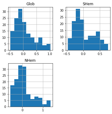
For example, we can draw a histogram of the column(s) in a DataFrame using the .hist method. For example:

dat[['Glob', 'SHem', 'NHem']].hist();

Line plots (`pandas`)#

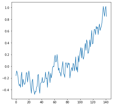
The .plot method, given a Series (or a DataFrame with one column), creates a line plot with the indices on the x-axis and the values on the y-axis:

dat['Glob'].plot();

In case we need to change the values on the x-axis, the simplest way is to set the required values as the index (see Modifying the index). For example, here we set the "Year" column as the DataFrame index, then plot the "Glob" column. As a result, the measurement year appears on the x-axis instead of the default consecutive index:

dat.set_index('Year')['Glob'].plot();

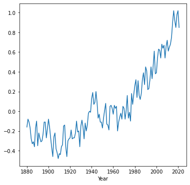
Pay attention to the order of operations (from left to right) in the above expression:

dat.set_index('Year')—Setting the index
['Glob']—Extracting a column (as Series)
.plot();—Plotting

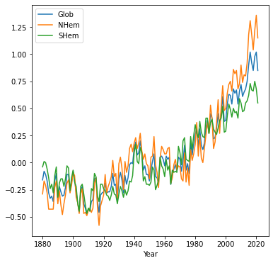
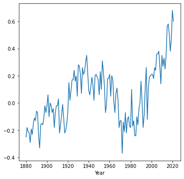
When we plot a DataFrame with more than one column, the columns are plotted as sepatate series in the same line plot. This is useful to compare the values in different columns. Fore example, plotting the "Glob", "NHem", and "SHem" columns demonstrates that in recent years Northern Hemisphere ("NHem") temperatures have been relatively higher, while Southern Hemisphere ("SHem") temperatures have been relatively lower, compared to the global average ("Glob"):

dat.set_index('Year')[['Glob', 'NHem', 'SHem']].plot();

Scatterplots (`pandas`)#

One more useful type of plot is a scatterplot, where we display the association between two series in the form of scattered points. To produce a scatterplot, we use the .plot.scatter method of a DataFrame, specifying the names of the columns to be displayed in the x-axis (x) and y-axis (y).

For example, the following expression shows the relation between the values in the 'NHem' and 'SHem' columns of dat:

dat.plot.scatter(x='NHem', y='SHem');

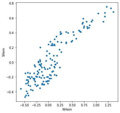
We clearly see that there is a strong positive association between Northern Hemisphere and Southern Hemisphere temperatures across years. Namely, in years when the Nothern Hemisphere temperature is high, the Southern Hemisphere temperature also tends to be high, and vice versa.

Operators#

Operators on `Series`#

Operators and summary functions can be applied to Series objects, similarly to the way they can be applied to numpy arrays (see Vectorized operations and Summarizing array values, respectively). For example, summary methods such as .min, .max, and .mean can be applied on a Series to summarize its respective properties. Here is how we can find out the start and end "Year" in dat:

dat['Year'].min()

dat['Year'].max()

and the average "Glob" value:

dat['Glob'].mean()

0.055633802816901445

We can also combine Series with individual values, or combine two series, to apply pairwise arithmetic or boolean operators. For example, here is how we can subtract 1 from all "Year" values:

dat['Year'] - 1

    1879
    1880
    1881
    1882
    1883
       ... 
  2016
  2017
  2018
  2019
  2020
Name: Year, Length: 142, dtype: int64

and here is how we can calculate the yearly differences between the Northern Hemisphere and Southern Hemisphere temperature anomalies:

dat['NHem'] - dat['SHem']

   -0.25
   -0.18
   -0.21
   -0.22
   -0.29
       ... 
  0.51
  0.38
  0.47
  0.68
  0.60
Length: 142, dtype: float64

Note that this is an arithmetic operation between two Series, which returns a new series.

Note

When performing operations between pairs of Series or DataFrames, pandas aligns the elements according to the index, rather than the position. When the data come from the same table (such as in the last example), the indices are guaranteed to match. However, when the data come from different tables, you must make sure their indices match.

Operators on `DataFrame`s#

Operating on an entire DataFrame is more complex than operating on a Series (see Operators on Series). Accordingly, operators behave in different ways. For example, arithmetic and boolean operations combined with an individual value are applied per-element, resulting in a new DataFrame (assuming that all columns are numeric):

dat - 10

	Year	Glob	NHem	SHem	24N-90N	...	EQU-24N	24S-EQU	44S-24S	64S-44S	90S-64S
0	1870	-10.16	-10.29	-10.04	-10.37	...	-10.15	-10.09	-10.03	-9.95	-9.35
1	1871	-10.08	-10.17	-9.99	-10.34	...	-9.90	-9.88	-10.05	-10.07	-9.43
2	1872	-10.11	-10.21	-10.00	-10.31	...	-10.05	-10.04	-9.98	-9.96	-9.40
3	1873	-10.17	-10.28	-10.06	-10.35	...	-10.17	-10.14	-10.03	-9.93	-9.52
4	1874	-10.28	-10.43	-10.14	-10.61	...	-10.13	-10.15	-10.19	-10.02	-9.37
...	...	...	...	...	...	...	...	...	...	...	...
137	2007	-9.08	-8.82	-9.33	-8.60	...	-9.13	-9.23	-9.24	-9.65	-9.45
138	2008	-9.15	-8.96	-9.34	-8.75	...	-9.27	-9.38	-9.21	-9.63	-9.04
139	2009	-9.02	-8.78	-9.25	-8.57	...	-9.09	-9.11	-9.26	-9.61	-9.17
140	2010	-8.98	-8.64	-9.32	-8.32	...	-9.11	-9.16	-9.42	-9.61	-9.09
141	2011	-9.15	-8.85	-9.45	-8.57	...	-9.27	-9.41	-9.29	-9.68	-9.67

142 rows × 15 columns

Methods such as .mean, however, are by default applied per column (i.e., axis=0):

dat.mean()

Year       1950.500000
Glob          0.055634
NHem          0.083169
SHem          0.028803
24N-90N       0.103732
              ...     
EQU-24N       0.054930
24S-EQU       0.079437
44S-24S       0.036127
64S-44S      -0.060704
90S-64S      -0.089507
Length: 15, dtype: float64

We elaborate on this type of row- and column-wise operations later on (see Row/col-wise operations).

Creating new columns#

New DataFrame columns can be created by assignment of a Series to a non-existing column index. For example, the following expression calculates a Series of yearly differences between the Northern Hemisphere and Southern Hemisphere temperatures, as shown above, and assigns it to a new column named diff:

dat['diff'] = dat['NHem'] - dat['SHem']
dat

	Year	Glob	NHem	SHem	24N-90N	...	24S-EQU	44S-24S	64S-44S	90S-64S	diff
0	1880	-0.16	-0.29	-0.04	-0.37	...	-0.09	-0.03	0.05	0.65	-0.25
1	1881	-0.08	-0.17	0.01	-0.34	...	0.12	-0.05	-0.07	0.57	-0.18
2	1882	-0.11	-0.21	0.00	-0.31	...	-0.04	0.02	0.04	0.60	-0.21
3	1883	-0.17	-0.28	-0.06	-0.35	...	-0.14	-0.03	0.07	0.48	-0.22
4	1884	-0.28	-0.43	-0.14	-0.61	...	-0.15	-0.19	-0.02	0.63	-0.29
...	...	...	...	...	...	...	...	...	...	...	...
137	2017	0.92	1.18	0.67	1.40	...	0.77	0.76	0.35	0.55	0.51
138	2018	0.85	1.04	0.66	1.25	...	0.62	0.79	0.37	0.96	0.38
139	2019	0.98	1.22	0.75	1.43	...	0.89	0.74	0.39	0.83	0.47
140	2020	1.02	1.36	0.68	1.68	...	0.84	0.58	0.39	0.91	0.68
141	2021	0.85	1.15	0.55	1.43	...	0.59	0.71	0.32	0.33	0.60

142 rows × 16 columns

Here is a plot (Line plots (pandas)) of the differences we just calulated, as function of time:

dat.set_index('Year')['diff'].plot();

We can also assign an expression that combines series with individual values:

dat['NHem2'] = dat['NHem'] * 2
dat

	Year	Glob	NHem	SHem	24N-90N	...	44S-24S	64S-44S	90S-64S	diff	NHem2
0	1880	-0.16	-0.29	-0.04	-0.37	...	-0.03	0.05	0.65	-0.25	-0.58
1	1881	-0.08	-0.17	0.01	-0.34	...	-0.05	-0.07	0.57	-0.18	-0.34
2	1882	-0.11	-0.21	0.00	-0.31	...	0.02	0.04	0.60	-0.21	-0.42
3	1883	-0.17	-0.28	-0.06	-0.35	...	-0.03	0.07	0.48	-0.22	-0.56
4	1884	-0.28	-0.43	-0.14	-0.61	...	-0.19	-0.02	0.63	-0.29	-0.86
...	...	...	...	...	...	...	...	...	...	...	...
137	2017	0.92	1.18	0.67	1.40	...	0.76	0.35	0.55	0.51	2.36
138	2018	0.85	1.04	0.66	1.25	...	0.79	0.37	0.96	0.38	2.08
139	2019	0.98	1.22	0.75	1.43	...	0.74	0.39	0.83	0.47	2.44
140	2020	1.02	1.36	0.68	1.68	...	0.58	0.39	0.91	0.68	2.72
141	2021	0.85	1.15	0.55	1.43	...	0.71	0.32	0.33	0.60	2.30

142 rows × 17 columns

or an individual value on its own (in which case it is duplicated across all rows):

dat['variable'] = 'temperature'
dat

	Year	Glob	NHem	SHem	24N-90N	...	64S-44S	90S-64S	diff	NHem2	variable
0	1880	-0.16	-0.29	-0.04	-0.37	...	0.05	0.65	-0.25	-0.58	temperature
1	1881	-0.08	-0.17	0.01	-0.34	...	-0.07	0.57	-0.18	-0.34	temperature
2	1882	-0.11	-0.21	0.00	-0.31	...	0.04	0.60	-0.21	-0.42	temperature
3	1883	-0.17	-0.28	-0.06	-0.35	...	0.07	0.48	-0.22	-0.56	temperature
4	1884	-0.28	-0.43	-0.14	-0.61	...	-0.02	0.63	-0.29	-0.86	temperature
...	...	...	...	...	...	...	...	...	...	...	...
137	2017	0.92	1.18	0.67	1.40	...	0.35	0.55	0.51	2.36	temperature
138	2018	0.85	1.04	0.66	1.25	...	0.37	0.96	0.38	2.08	temperature
139	2019	0.98	1.22	0.75	1.43	...	0.39	0.83	0.47	2.44	temperature
140	2020	1.02	1.36	0.68	1.68	...	0.39	0.91	0.68	2.72	temperature
141	2021	0.85	1.15	0.55	1.43	...	0.32	0.33	0.60	2.30	temperature

142 rows × 18 columns

Let us delete the 'diff', 'NHem2', 'variable' columns we just created to get the original version of dat:

dat = dat.drop(['diff', 'NHem2', 'variable'], axis=1)
dat

	Year	Glob	NHem	SHem	24N-90N	...	EQU-24N	24S-EQU	44S-24S	64S-44S	90S-64S
0	1880	-0.16	-0.29	-0.04	-0.37	...	-0.15	-0.09	-0.03	0.05	0.65
1	1881	-0.08	-0.17	0.01	-0.34	...	0.10	0.12	-0.05	-0.07	0.57
2	1882	-0.11	-0.21	0.00	-0.31	...	-0.05	-0.04	0.02	0.04	0.60
3	1883	-0.17	-0.28	-0.06	-0.35	...	-0.17	-0.14	-0.03	0.07	0.48
4	1884	-0.28	-0.43	-0.14	-0.61	...	-0.13	-0.15	-0.19	-0.02	0.63
...	...	...	...	...	...	...	...	...	...	...	...
137	2017	0.92	1.18	0.67	1.40	...	0.87	0.77	0.76	0.35	0.55
138	2018	0.85	1.04	0.66	1.25	...	0.73	0.62	0.79	0.37	0.96
139	2019	0.98	1.22	0.75	1.43	...	0.91	0.89	0.74	0.39	0.83
140	2020	1.02	1.36	0.68	1.68	...	0.89	0.84	0.58	0.39	0.91
141	2021	0.85	1.15	0.55	1.43	...	0.73	0.59	0.71	0.32	0.33

142 rows × 15 columns

`DataFrame` filtering#

Using conditional operators#

Most often, instead of selecting rows by index or by position (see Selecting DataFrame rows), we want to filter rows by a condition that we apply on table values. For example, suppose that we want to get a subset of dat with all rows after the year 2017. To do that, we can create a boolean Series, specifying which rows are to be retained:

sel = dat['Year'] > 2017
sel

    False
    False
    False
    False
    False
       ...  
  False
   True
   True
   True
   True
Name: Year, Length: 142, dtype: bool

Then, the boolean series can be passed as an index inside square brackets ([), to select those rows corresponding to True:

dat[sel]

	Year	Glob	NHem	SHem	24N-90N	...	EQU-24N	24S-EQU	44S-24S	64S-44S	90S-64S
138	2018	0.85	1.04	0.66	1.25	...	0.73	0.62	0.79	0.37	0.96
139	2019	0.98	1.22	0.75	1.43	...	0.91	0.89	0.74	0.39	0.83
140	2020	1.02	1.36	0.68	1.68	...	0.89	0.84	0.58	0.39	0.91
141	2021	0.85	1.15	0.55	1.43	...	0.73	0.59	0.71	0.32	0.33

4 rows × 15 columns

The same can be acheived in a single step, without storing the Series in a variable such as sel, as follows:

dat[dat['Year'] > 2017]

	Year	Glob	NHem	SHem	24N-90N	...	EQU-24N	24S-EQU	44S-24S	64S-44S	90S-64S
138	2018	0.85	1.04	0.66	1.25	...	0.73	0.62	0.79	0.37	0.96
139	2019	0.98	1.22	0.75	1.43	...	0.91	0.89	0.74	0.39	0.83
140	2020	1.02	1.36	0.68	1.68	...	0.89	0.84	0.58	0.39	0.91
141	2021	0.85	1.15	0.55	1.43	...	0.73	0.59	0.71	0.32	0.33

4 rows × 15 columns

Exercise 05-e

Create a subset of dat with all rows where the global temperature anomaly ('Glob') was above 1 degree.

Using `.isin`#

Sometimes, the condition we are interested in is not a comparison against an individual value (such as >2017, see Using conditional operators), but multiple values. For example, suppose we want to extract the rows corresponding to the years 2008, 2012, and 2016, in dat. One way is to compose a combined condition using |, using the numpy syntax we are familiar with (see numpy conditional operators). Again, recall that we must enclose each internal expression in breackets ( so that it is evaluated before |:

sel = (dat['Year'] == 2008) | (dat['Year'] == 2012) | (dat['Year'] == 2016)
dat[sel]

	Year	Glob	NHem	SHem	24N-90N	...	EQU-24N	24S-EQU	44S-24S	64S-44S	90S-64S
128	2008	0.54	0.68	0.41	0.92	...	0.34	0.42	0.52	0.09	0.62
132	2012	0.65	0.81	0.48	1.04	...	0.48	0.57	0.56	0.19	0.41
136	2016	1.02	1.31	0.73	1.55	...	0.96	1.06	0.67	0.25	0.41

3 rows × 15 columns

As you can imagine, this method quickly becomes unfeasible if the number of items becomes large. Instead, we can use the .isin method, combined with a list of items to compare with the Series values:

sel = dat['Year'].isin([2008, 2012, 2016])
dat[sel]

	Year	Glob	NHem	SHem	24N-90N	...	EQU-24N	24S-EQU	44S-24S	64S-44S	90S-64S
128	2008	0.54	0.68	0.41	0.92	...	0.34	0.42	0.52	0.09	0.62
132	2012	0.65	0.81	0.48	1.04	...	0.48	0.57	0.56	0.19	0.41
136	2016	1.02	1.31	0.73	1.55	...	0.96	1.06	0.67	0.25	0.41

3 rows × 15 columns

Recall the in operator which we learned about earlier (see The in operator). The in operator is analogous to the .isin method, but intended for lists.

Exercise 05-f

What do you think is the meaning of dat[~sel]? Try it to check your answer.

Assignment to subsets#

When assigning to subsets of a column, we need to use the .loc method. Typically we combine:

A boolean Series in the rows index, to select the observations we want to modify
A single string in the columns index, to select the variable we want to modify

For example, the following expression sets the 'NHem' column value to 12.3 in all years after 2017:

dat.loc[dat['Year'] > 2017, 'NHem'] = 999
dat

	Year	Glob	NHem	SHem	24N-90N	...	EQU-24N	24S-EQU	44S-24S	64S-44S	90S-64S
0	1880	-0.16	-0.29	-0.04	-0.37	...	-0.15	-0.09	-0.03	0.05	0.65
1	1881	-0.08	-0.17	0.01	-0.34	...	0.10	0.12	-0.05	-0.07	0.57
2	1882	-0.11	-0.21	0.00	-0.31	...	-0.05	-0.04	0.02	0.04	0.60
3	1883	-0.17	-0.28	-0.06	-0.35	...	-0.17	-0.14	-0.03	0.07	0.48
4	1884	-0.28	-0.43	-0.14	-0.61	...	-0.13	-0.15	-0.19	-0.02	0.63
...	...	...	...	...	...	...	...	...	...	...	...
137	2017	0.92	1.18	0.67	1.40	...	0.87	0.77	0.76	0.35	0.55
138	2018	0.85	999.00	0.66	1.25	...	0.73	0.62	0.79	0.37	0.96
139	2019	0.98	999.00	0.75	1.43	...	0.91	0.89	0.74	0.39	0.83
140	2020	1.02	999.00	0.68	1.68	...	0.89	0.84	0.58	0.39	0.91
141	2021	0.85	999.00	0.55	1.43	...	0.73	0.59	0.71	0.32	0.33

142 rows × 15 columns

To get back to the original values, let us read the CSV file once again:

dat = pd.read_csv('data/ZonAnn.Ts+dSST.csv')
dat

	Year	Glob	NHem	SHem	24N-90N	...	EQU-24N	24S-EQU	44S-24S	64S-44S	90S-64S
0	1880	-0.16	-0.29	-0.04	-0.37	...	-0.15	-0.09	-0.03	0.05	0.65
1	1881	-0.08	-0.17	0.01	-0.34	...	0.10	0.12	-0.05	-0.07	0.57
2	1882	-0.11	-0.21	0.00	-0.31	...	-0.05	-0.04	0.02	0.04	0.60
3	1883	-0.17	-0.28	-0.06	-0.35	...	-0.17	-0.14	-0.03	0.07	0.48
4	1884	-0.28	-0.43	-0.14	-0.61	...	-0.13	-0.15	-0.19	-0.02	0.63
...	...	...	...	...	...	...	...	...	...	...	...
137	2017	0.92	1.18	0.67	1.40	...	0.87	0.77	0.76	0.35	0.55
138	2018	0.85	1.04	0.66	1.25	...	0.73	0.62	0.79	0.37	0.96
139	2019	0.98	1.22	0.75	1.43	...	0.91	0.89	0.74	0.39	0.83
140	2020	1.02	1.36	0.68	1.68	...	0.89	0.84	0.58	0.39	0.91
141	2021	0.85	1.15	0.55	1.43	...	0.73	0.59	0.71	0.32	0.33

142 rows × 15 columns

Working with missing data (`pandas`)#

Missing data in `pandas`#

Missing values, denoting that the true value is unknown, are an inevitable feature of real-world data. In plain-text formats, such as CSV, missing values are commonly just “missing”, i.e., left blank, or marked with a labels such as the text "NA".

Treatment of “No Data” values in Series and DataFrames is derived from the underlying behavior in numpy (Working with missing data (numpy)), as pandas is based on numpy. Namely, “No Data” values are typically represented using np.nan.

pandas may automatically transform the Series data type, and “No Data” representation, for optimized data storage. For example, a Series of type int which contains one or more np.nan value, is automatically transformed to float, similarly to the behaviour we have seen with numpy array (Working with missing data (numpy)):

pd.Series([7, 4, 3])

  7
  4
  3
dtype: int64

pd.Series([7, np.nan, 3])

  7.0
  NaN
  3.0
dtype: float64

Moreover, None values are automatically transformed to np.nan (unlike numpy, where None values are preserved, resulting in an object array):

pd.Series([7, None, 3])

  7.0
  NaN
  3.0
dtype: float64

“No Data” values are automatically assigned where necessary when creating a Series or a DataFrame through other methods too. For example, empty cells in a CSV file are assigned with np.nan when importing the CSV into a DataFrame (see Reading from file).

The students.csv file contains annual students counts in universities of Israel during the period 1969-2020:

The first column ("year") specifies the academic year
All other columns (Ariel University", "Weizmann Institute of Science", etc.) represent the different universities and their student counts

If you open the CSV file in a spreadsheet program (such as Excel), you will see that some of the cells are empty. Those cells are assigned with np.nan when importing the table:

students = pd.read_csv('data/students.csv')
students

	year	Ariel University	Weizmann Institute of Science	Ben-Gurion Univ. of the Negev	Haifa University	Bar-Ilan University	Tel-Aviv University	Technion	Hebrew University
0	1969/70	NaN	419.0	1297	2794	4273	7958	6045	12588
1	1974/75	NaN	580.0	3247	4713	6527	12813	8453	13516
2	1979/80	NaN	490.0	4250	6140	8070	14380	7580	13570
3	1980/81	NaN	NaN	4430	6040	8670	14860	7620	13770
4	1981/82	NaN	NaN	4500	6055	8730	15770	7650	14000
...	...	...	...	...	...	...	...	...	...
38	2015/16	10977.0	1104.0	17918	18027	20621	26643	14240	20171
39	2016/17	NaN	NaN	17797	18047	18830	26342	14501	19784
40	2017/18	11899.0	NaN	17724	17471	17523	26023	14054	19582
41	2018/19	11741.0	1148.0	17699	17570	17340	26361	13611	19837
42	2019/20	12016.0	1215.0	17820	17396	17764	26570	13787	20898

43 rows × 9 columns

For example, the first value in the "Ariel University" column is missing:

students['Ariel University'].iloc[0]

nan

Detecting with `pd.isna`#

To detect “No Data” values, the .isna method (or pd.isna function) can be applied on a Series or a DataFrame. The result is a boolean mask that marks the missing values. The pd.isna function from pandas is analogous to the np.isnan function for arrays, which we learned about earlier (see Detecting “No Data” (np.isnan)).

For example, students.isna() returns a boolean DataFrame, of the same shape as students, with True marking “No Data” values:

students.isna()

	year	Ariel University	Weizmann Institute of Science	Ben-Gurion Univ. of the Negev	Haifa University	Bar-Ilan University	Tel-Aviv University	Technion	Hebrew University
0	False	True	False	False	False	False	False	False	False
1	False	True	False	False	False	False	False	False	False
2	False	True	False	False	False	False	False	False	False
3	False	True	True	False	False	False	False	False	False
4	False	True	True	False	False	False	False	False	False
...	...	...	...	...	...	...	...	...	...
38	False	False	False	False	False	False	False	False	False
39	False	True	True	False	False	False	False	False	False
40	False	False	True	False	False	False	False	False	False
41	False	False	False	False	False	False	False	False	False
42	False	False	False	False	False	False	False	False	False

43 rows × 9 columns

Similarly, the .isna() method applied on a Series returns a new boolean Series where “No Data” values are marked with True:

students['Ariel University'].isna()

    True
    True
    True
    True
    True
      ...  
  False
   True
  False
  False
  False
Name: Ariel University, Length: 43, dtype: bool

The ~ operator (see numpy conditional operators) reverses a boolean Series. This is very useful in the context of “No Data” masks, since it can reverse the mask so that it points at non-missing values.

For example, here is how we can get the reverse of students.isna():

~students.isna()

	year	Ariel University	Weizmann Institute of Science	Ben-Gurion Univ. of the Negev	Haifa University	Bar-Ilan University	Tel-Aviv University	Technion	Hebrew University
0	True	False	True	True	True	True	True	True	True
1	True	False	True	True	True	True	True	True	True
2	True	False	True	True	True	True	True	True	True
3	True	False	False	True	True	True	True	True	True
4	True	False	False	True	True	True	True	True	True
...	...	...	...	...	...	...	...	...	...
38	True	True	True	True	True	True	True	True	True
39	True	False	False	True	True	True	True	True	True
40	True	True	False	True	True	True	True	True	True
41	True	True	True	True	True	True	True	True	True
42	True	True	True	True	True	True	True	True	True

43 rows × 9 columns

and here is how we can get the reverse of students['Ariel University'].isna():

~students['Ariel University'].isna()

   False
   False
   False
   False
   False
      ...  
   True
  False
   True
   True
   True
Name: Ariel University, Length: 43, dtype: bool

Another possible use of ~ and .isna is to extract the non-missing values from a series. Here is an example:

students['Ariel University'][~students['Ariel University'].isna()]

  10977.0
  11899.0
  11741.0
  12016.0
Name: Ariel University, dtype: float64

However, there is a dedicated method called .dropna to do that with shorter code (see Removing with .dropna):

students['Ariel University'].dropna()

  10977.0
  11899.0
  11741.0
  12016.0
Name: Ariel University, dtype: float64

Similarly, we can extract DataFrame rows where a particular column is non-missing. For example, here we have those students rows that have a valid 'Ariel University' student count:

students[~students['Ariel University'].isna()]

	year	Ariel University	Weizmann Institute of Science	Ben-Gurion Univ. of the Negev	Haifa University	Bar-Ilan University	Tel-Aviv University	Technion	Hebrew University
38	2015/16	10977.0	1104.0	17918	18027	20621	26643	14240	20171
40	2017/18	11899.0	NaN	17724	17471	17523	26023	14054	19582
41	2018/19	11741.0	1148.0	17699	17570	17340	26361	13611	19837
42	2019/20	12016.0	1215.0	17820	17396	17764	26570	13787	20898

Note

Instead of reversing the output of pd.isna with the ~operator, another option is to use the inverse method .notna, which returns the non-missing mask.

Finally, it is often useful to combine the .isna method with .any to find out if a Series contains at least one missing value:

students['Ariel University'].isna().any()

True

students['Ben-Gurion Univ. of the Negev'].isna().any()

False

or to find out which columns contain at least one missing value:

students.isna().any()

year                             False
Ariel University                  True
Weizmann Institute of Science     True
Ben-Gurion Univ. of the Negev    False
Haifa University                 False
Bar-Ilan University              False
Tel-Aviv University              False
Technion                         False
Hebrew University                False
dtype: bool

We can also use .sum to find out how many missing value are there in each column:

students.isna().sum()

year                              0
Ariel University                 39
Weizmann Institute of Science     6
Ben-Gurion Univ. of the Negev     0
Haifa University                  0
Bar-Ilan University               0
Tel-Aviv University               0
Technion                          0
Hebrew University                 0
dtype: int64

Operators with missing values#

When applying a method such as .sum, .mean, .min, or .max (or the respective np.* function) on a Series, the “No Data” values are ignored. That is, the result is based only on the non-missing values. For example:

students['Ariel University'].sum()

46633.0

Note that this behavior is specific to pandas, and unlike what we have seen with numpy arrays, where these opertions return “No Data” if at least one of the values in the array is “No Data” (see Operations with “No Data”):

students['Ariel University'].to_numpy().sum()

nan

Element-by-element operations, however, expectedly result in “No Data” when applied to “No Data” elements, since the result cannot be computed at all. For example:

students['Ariel University'] / 1000

      NaN
      NaN
      NaN
      NaN
      NaN
       ...  
  10.977
     NaN
  11.899
  11.741
  12.016
Name: Ariel University, Length: 43, dtype: float64

Removing with `.dropna`#

The .dropna method can be used to remove missing values from a DataFrame (or a Series). The default is to drop all rows that have at least one missing value, i.e., keeping only complete observations. For example:

students.dropna()

	year	Ariel University	Weizmann Institute of Science	Ben-Gurion Univ. of the Negev	Haifa University	Bar-Ilan University	Tel-Aviv University	Technion	Hebrew University
38	2015/16	10977.0	1104.0	17918	18027	20621	26643	14240	20171
41	2018/19	11741.0	1148.0	17699	17570	17340	26361	13611	19837
42	2019/20	12016.0	1215.0	17820	17396	17764	26570	13787	20898

Note

There are other parameters of .dropna for dropping columns instead of rows, or dropping rows or column using a threshold of “acceptable” minimum number of non-missing values. See the documentation for details: https://pandas.pydata.org/docs/reference/api/pandas.DataFrame.dropna.html.

Replacing with `.fillna`#

Missing values can be replaced using the .fillna method. The parameter specifies which new value should be placed instead of the “No Data” values. For example, here is how we can replace the “No Data” values in the "Ariel University" student counts column with 0:

students['Ariel University'].fillna(0)

       0.0
       0.0
       0.0
       0.0
       0.0
       ...   
  10977.0
      0.0
  11899.0
  11741.0
  12016.0
Name: Ariel University, Length: 43, dtype: float64

or assign the result back to the students table:

students['Ariel University'] = students['Ariel University'].fillna(0)
students

	year	Ariel University	Weizmann Institute of Science	Ben-Gurion Univ. of the Negev	Haifa University	Bar-Ilan University	Tel-Aviv University	Technion	Hebrew University
0	1969/70	0.0	419.0	1297	2794	4273	7958	6045	12588
1	1974/75	0.0	580.0	3247	4713	6527	12813	8453	13516
2	1979/80	0.0	490.0	4250	6140	8070	14380	7580	13570
3	1980/81	0.0	NaN	4430	6040	8670	14860	7620	13770
4	1981/82	0.0	NaN	4500	6055	8730	15770	7650	14000
...	...	...	...	...	...	...	...	...	...
38	2015/16	10977.0	1104.0	17918	18027	20621	26643	14240	20171
39	2016/17	0.0	NaN	17797	18047	18830	26342	14501	19784
40	2017/18	11899.0	NaN	17724	17471	17523	26023	14054	19582
41	2018/19	11741.0	1148.0	17699	17570	17340	26361	13611	19837
42	2019/20	12016.0	1215.0	17820	17396	17764	26570	13787	20898

43 rows × 9 columns

Let us return to the original students table by converting the cells back to “No Data”:

students.loc[students['Ariel University'] == 0, 'Ariel University'] = np.nan
students

	year	Ariel University	Weizmann Institute of Science	Ben-Gurion Univ. of the Negev	Haifa University	Bar-Ilan University	Tel-Aviv University	Technion	Hebrew University
0	1969/70	NaN	419.0	1297	2794	4273	7958	6045	12588
1	1974/75	NaN	580.0	3247	4713	6527	12813	8453	13516
2	1979/80	NaN	490.0	4250	6140	8070	14380	7580	13570
3	1980/81	NaN	NaN	4430	6040	8670	14860	7620	13770
4	1981/82	NaN	NaN	4500	6055	8730	15770	7650	14000
...	...	...	...	...	...	...	...	...	...
38	2015/16	10977.0	1104.0	17918	18027	20621	26643	14240	20171
39	2016/17	NaN	NaN	17797	18047	18830	26342	14501	19784
40	2017/18	11899.0	NaN	17724	17471	17523	26023	14054	19582
41	2018/19	11741.0	1148.0	17699	17570	17340	26361	13611	19837
42	2019/20	12016.0	1215.0	17820	17396	17764	26570	13787	20898

43 rows × 9 columns

Copies#

One more thing we need to be aware when working with pandas is the distinction between references and copies. The pandas package (and geopandas which extends it, see Vector layers (geopandas)) behaves similarly to numpy with respect to copies (see Views and copies). We must be aware of whether we are creating a view or a copy of a DataFrame, to avoid unexpected results.

Here is a small demonstration, very similar to the one we did with numpy arrays (see Views and copies). Suppose that we create a copy of dat, named dat2:

dat2 = dat

Next, we modify dat2, assigning a new value such as 9999 into a particular cell (e.g., 2^nd row, 2^nd column):

dat2.iloc[1, 1] = 9999

The printout of the table top-left “corner” demonstrates the value was actually changed:

dat2.iloc[:4, :4]

	Year	Glob	NHem	SHem
0	1880	-0.16	-0.29	-0.04
1	1881	9999.00	-0.17	0.01
2	1882	-0.11	-0.21	0.00
3	1883	-0.17	-0.28	-0.06

What may be surprising, again, is that the original table dat has also changed. We thus demonstrated that dat2 is a reference to dat, rather than an independent copy:

dat.iloc[:4, :4]

	Year	Glob	NHem	SHem
0	1880	-0.16	-0.29	-0.04
1	1881	9999.00	-0.17	0.01
2	1882	-0.11	-0.21	0.00
3	1883	-0.17	-0.28	-0.06

To create an independent copy, so that its modifications are not reflected in the original, we need to explicitly use the .copy method, as in:

dat2 = dat.copy()

Let us read the CSV file again to get back to the original values:

dat = pd.read_csv('data/ZonAnn.Ts+dSST.csv')

Writing to file#

A DataFrame can be exported to several formats, such as CSV, using the appropriate method. For example, exporting to CSV is done using the .to_csv method.

Here is how we can export the DataFrame named stations, which we created in the beginning of the chapter (see Creating a DataFrame), to a CSV file named stations.csv in the output directory. The additional index=False argument specifies that we do not want to export the index values, which is usually the case:

stations.to_csv('output/stations.csv', index=False)

Note that the file is exported to a sub-directory named output (which must already exist!).

The way the resulting file stations.csv is displayed in a spreadsheet program, such as Microsoft Excel or LibreOffice Calc, is shown in Fig. 28.

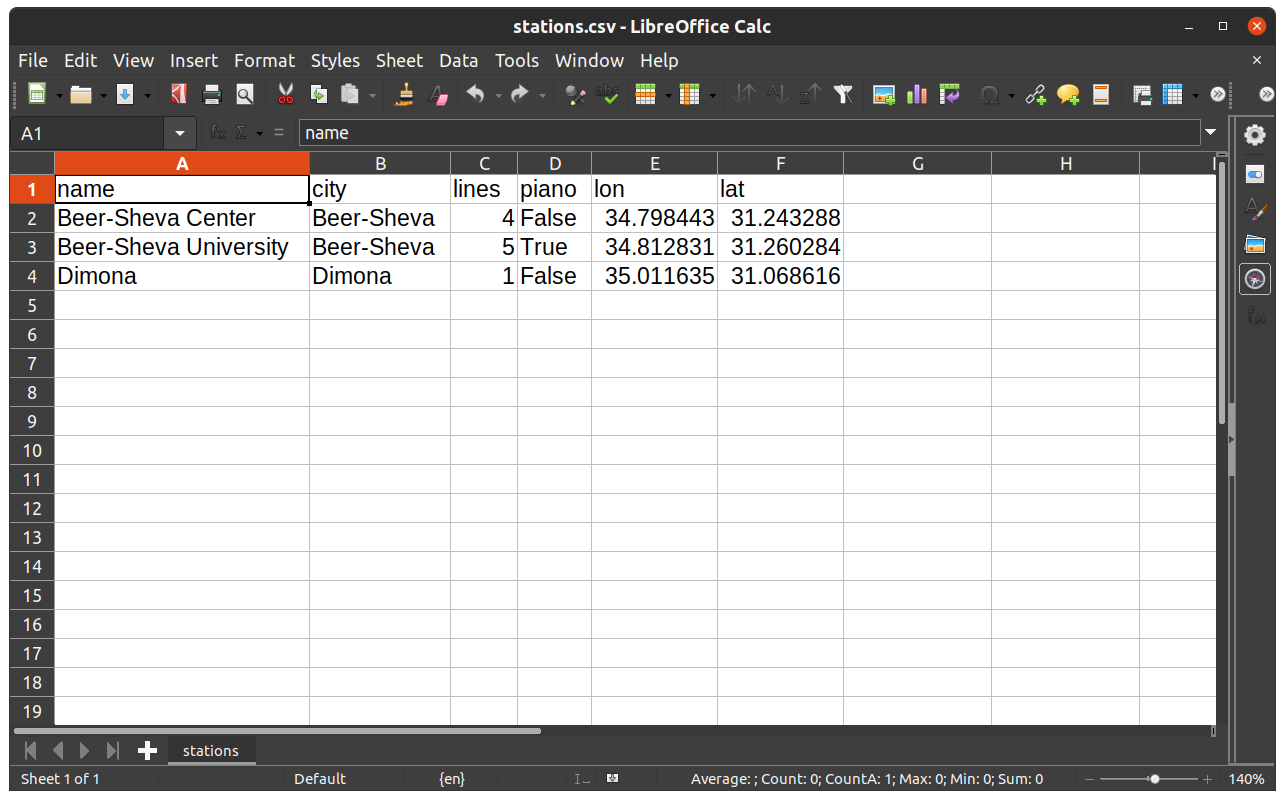
_images/exported_csv.png — Fig. 28 The `DataFrame` named `stations` when exported to CSV file and opened in LibreOffice Calc#

More exercises#

Exercise 05-g

Import the file students.csv into a DataFrame.
Calculate the total number of students in "Ben-Gurion Univ. of the Negev" across all years. (answer: 543615)
Calculate the total number of students enrolled in "Ariel University" across all years. (answer: 46633.0)
Use the expression given below to transform the "year" column to a numeric column specifying the year when the term ends (e.g., "2003/04" becomes 2004).
What is the range of observed years? Place the result into a list, and print it. (answer: [1970,2020])
In what year was the highest number of students in "Ben-Gurion Univ. of the Negev"? (answer: 2011)
In what year was the highest number of students in the "Weizmann Institute of Science"? (answer: 2020)

students["year"] = pd.to_numeric(students["year"].str.split("/").str[0]) + 1

Exercise 05-h

Read the file kinneret_level.csv to a DataFrame object named kinneret. The file contains daily measurements of the water level in Lake Kinneret. Note that water level was not measured on all days. Days with no measurements were not recorded in the file.
Rename the columns to 'date' and 'value', which are easier to work with.
Use the code given below to fill “missing” days with np.nan, so that the time-series is complete. Note that now the table has one column named value, while the (now consecutive) dates are stored in a special index of type DatetimeIndex (see https://stackoverflow.com/questions/19324453/add-missing-dates-to-pandas-dataframe#answer-19324591).
Plot the water level time series.
Calculate the proportion of days without a water level measurement (answer: 0.5348905538416336).
What was the lowest water level observed? On which day(s) was it observed? Hint: compare the minimum value with the entire series, then use the resulting boolean Series to filter table rows.
What was the longest consecutive period without a measurement? Hint: use a loop that goes over the table rows, and increment a counter variable whenever the current water level is “No Data”; when the current value isn’t “No Data”, (1) reset the counter variable, and (2) keep the current record if it’s highest, or else replace the current record (answer: 245).

kinneret['date'] = pd.to_datetime(kinneret['date'])
dates = pd.date_range(kinneret['date'].min(), kinneret['date'].max())
kinneret = kinneret.set_index('date')
kinneret = kinneret.reindex(dates, fill_value = np.nan)

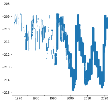
_images/exercise_solutions_pandas1_18_0.png — Fig. 29 Kinneret water level time series, from the solution of exercise-05-h#

Spatial Data Programming with Python

Tables (pandas)

Contents

Tables (pandas)#

Introduction#

What is pandas?#

Creating from scratch#

Creating a Series#

Creating a DataFrame#

Reading from file#

DataFrame properties#

Overview#

DataFrame dimensions#

DataFrame column names#

DataFrame column types#

Renaming columns#

Subsetting in pandas#

Subsetting Series#

Subsetting DataFrames#

Selecting DataFrame columns#

Selecting DataFrame rows#

Selecting rows and columns#

Selecting DataFrame values#

Convertsion to ndarray#

Conversion to list#

Series to list#

DataFrame to list#

Modifying the index#

Overivew#

Setting Series index#

Setting DataFrame index#

Resetting the index#

Sorting#

Plotting (pandas)#

Histograms (pandas)#

Line plots (pandas)#

Scatterplots (pandas)#

Operators#

Operators on Series#

Operators on DataFrames#

Creating new columns#

DataFrame filtering#

Using conditional operators#

Using .isin#

Assignment to subsets#

Working with missing data (pandas)#

Missing data in pandas#

Detecting with pd.isna#

Operators with missing values#

Removing with .dropna#

Replacing with .fillna#

Copies#

Writing to file#

More exercises#

Tables (`pandas`)#

What is `pandas`?#

Creating a `Series`#

Creating a `DataFrame`#

`DataFrame` properties#

`DataFrame` dimensions#

`DataFrame` column names#

`DataFrame` column types#

Subsetting in `pandas`#

Subsetting `Series`#

Subsetting `DataFrame`s#

Selecting `DataFrame` columns#

Selecting `DataFrame` rows#

Selecting `DataFrame` values#

Convertsion to `ndarray`#

Conversion to `list`#

`Series` to `list`#

`DataFrame` to `list`#

Setting `Series` index#

Setting `DataFrame` index#

Plotting (`pandas`)#

Histograms (`pandas`)#

Line plots (`pandas`)#

Scatterplots (`pandas`)#

Operators on `Series`#

Operators on `DataFrame`s#

`DataFrame` filtering#

Using `.isin`#

Working with missing data (`pandas`)#

Missing data in `pandas`#

Detecting with `pd.isna`#

Removing with `.dropna`#

Replacing with `.fillna`#