Setting up the environment

Last updated: 2024-02-24 18:02:31

---

Introduction

In this chapter we cover the prerequisites to setup the Python environment and interface, before we start with actually learning the Python language in the next chapters. Specifically, before starting to write Python code, you need to install and learn how to use several software components:

• Miniconda, which is a popular Python package manager, and includes the Python program itself (see Installing Miniconda and Using the Miniconda command line)

• Jupyter Notebook, the de-facto standard editor for writing and executing Python code in the data science domain, installed from within Miniconda (see Jupyter Notebook and Working with notebooks)

• Several Python packages, most importantly numpy, pandas, shapely, geopandas, and rasterio, which we are going to use in later chapters to work with arrays, tables, vector layers and rasters (see Python packages), also installed from within Miniconda

We also cover the concept of file paths (see File paths), which is essential for importing and exporting data from files in your Python scripts.

Running Python code

Python setup

Python is an interpreted programming language. This means that the expressions we write in the Python language are executed one by one by the software component known as the interpreter. This is unlike complied languages, which are more difficult to work with, such as the C language, where the entire script needs to be translated to an executable file before it can be run. In an interpreted language, however, the interpreter runs one expression at a time, returning the results or performing other operations (such as writing to a file) as it goes along our code.

There are several types of working environments that facilitate writing and running Python code. The common feature of all those environments is that they communicate with the Python interpreter. However, each environment also has other features that facilitate writing code and viewing the results. Python working environments include The Python command line, IPython, and Jupyter Notebook.

The Python program itself, as well as the environments used to access it and manage its packages (Python packages), are bundled into various software packages, also known as distributions. For example, Python can be downloaded and installed as a minimalist standalone program (Fig. 1), or as part of a package management system, such as Anaconda or Miniconda. Python is also commonly incorporated into other software installations, including GIS software such as QGIS, ArcGIS or ArcPro, where it can be accessed through an internal command line (ArcGIS Pro scripting (arcpy)). Finally, Mac OS and Linux typically come with a built-in, “system”, Python installation.

Python setup methods and environemnts are notoriously variable, whereas multiple Python versions on the same computer may conflict and “break” (Fig. 6). In this chapter we aim to use one of the simplest and safest methods, based on Miniconda.

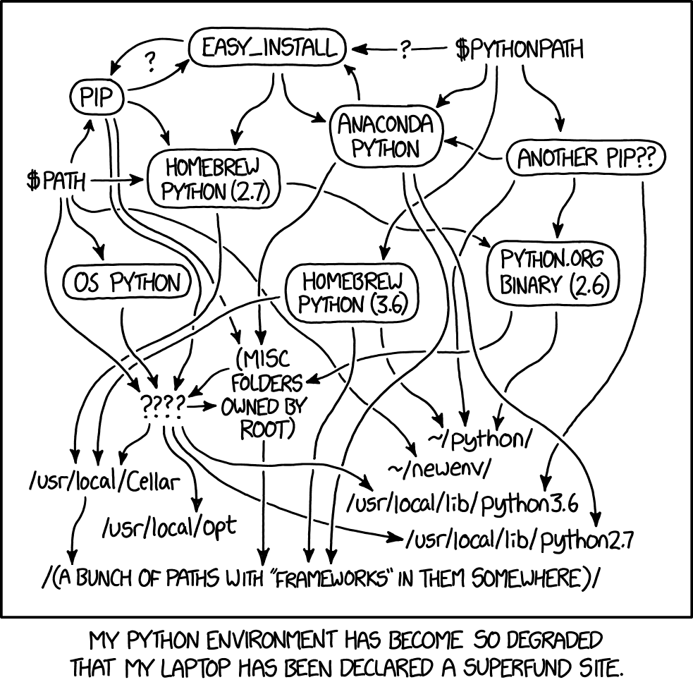
Fig. 6 Setting up Python (source: https://xkcd.com/1987/)

What software will we use?

In this chapter, we cover the software components that we are going to use for the rest of the book (except for the last chapter, ArcGIS Pro scripting (arcpy)).

The main component we are going to use is the Miniconda software. Miniconda is the recommended way to install Python on your computer for the purposes described in this book. Miniconda is the minimalist version of the well-known Anaconda software. Miniconda includes just Python, the conda package manager for Python (see Installing packages), and few other packages, whereas Anaconda comes with over 250 pre-installed Python packages. However, the pre-installed packages in Anaconda do not include most spatial packages we are going to need.

All software components we need other than Miniconda, namely Jupyter Notebook and other Python packages, can be installed through the Miniconda command line. Therefore, a prerequisite to the following material is that you have Miniconda installed (see Installing Miniconda), that you have access to the Miniconda command prompt (Fig. 9), and that you can run Miniconda as administrator to install the required packages (see Installing packages), or you have those packages already installed (e.g., by the IT administrator).

It is important to note that Python, Miniconda, and the third-party Python packages we are going to use in this book are free and open-source. Therefore, you can flexibly use the material we are going to learn, later on in your carreer, in any setting and at no cost: at work in a commercial company, at a university, in personal projects at home, and so on.

In the last chapter, we are going to use Python to automate a commercial software called ArcGIS Pro (see ArcGIS Pro scripting (arcpy)). ArcGIS Pro is paid software, and its installation and use is beyond the scope of this book. This chapter is intended for readers who are already working with ArcGIS Pro and would like to get a taste of enhancing their workflow using Python.

The instructions in this chapter assume the Windows 10 operating system.

Installing Miniconda

To install Miniconda, go to the Miniconda downloads section (Fig. 7), choose the right installation file for your system (such as Miniconda3 Windows 64-bit, download the file and execute it to run the installation process.

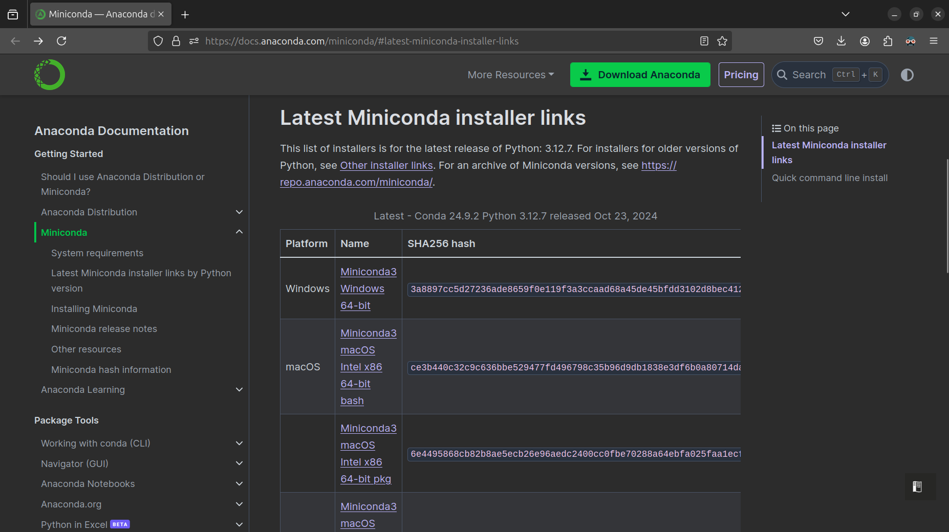
Fig. 7 The Miniconda website with download links

Note

Check out https://autogis-site.readthedocs.io/en/latest/course-info/installing-python.html for another tutorial of the setup we go through in this chapter, namely installing Miniconda (see Installing Miniconda) and Python packages (see Installing packages).

Using the Miniconda command line

The Miniconda command line

To start the Miniconda command line, locate the Anaconda Prompt (Miniconda3) entry in your Start menu (Fig. 8), and click on it.

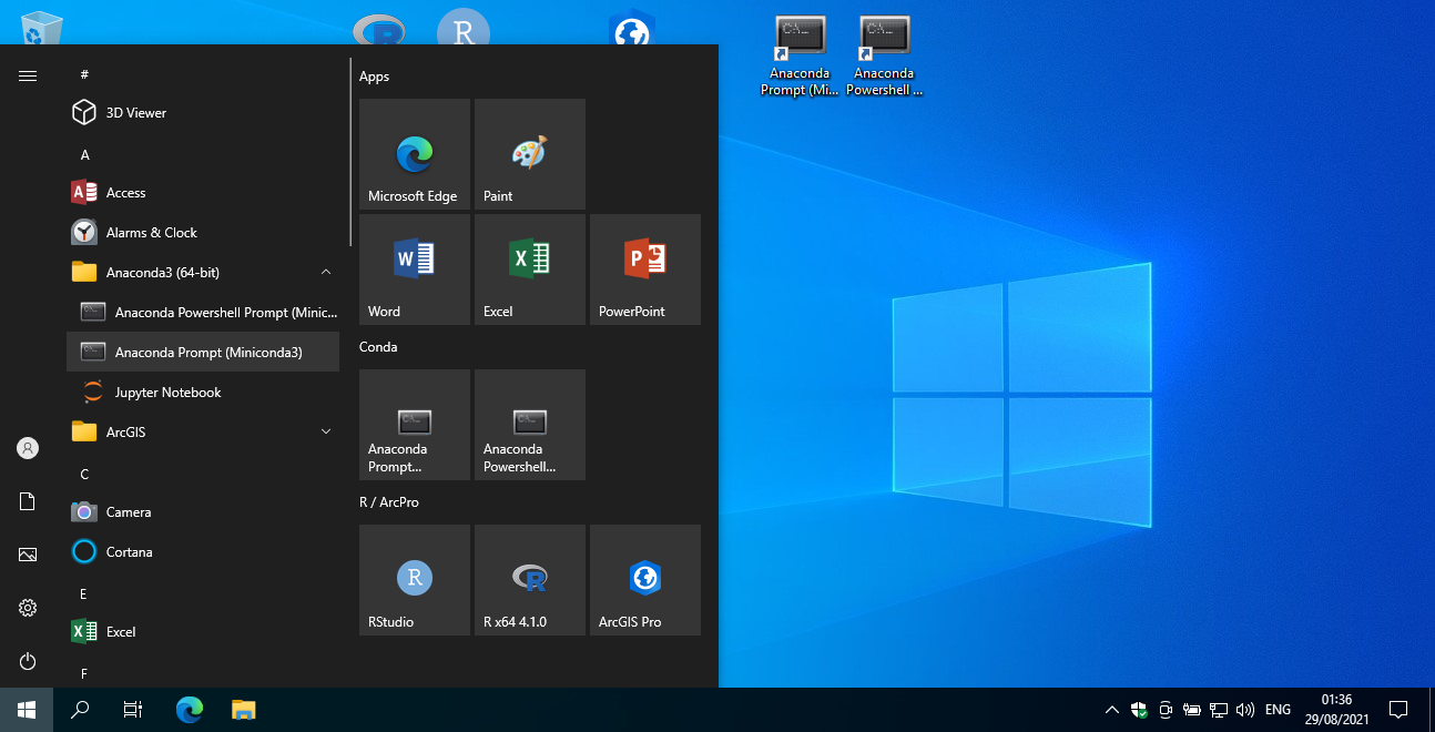
Fig. 8 The “Anaconda Prompt (Miniconda3)” icon to start the Miniconda prompt.

You should see a command line window (Fig. 9). Just like in any command-line interface, you can type and execute commands. For the purposes of this book, you need to be familiar with the following commands:

• Commands to move through drives and directories:

  • cd—Short for “change directory”, to move through the directory structure (in the same drive), as in cd C:\Users\dorman\Downloads

  • X:—To switch to a different drive, type the drive name followed by colon, as in D: to switch to drive D:\

  • dir—To list current directory contents

• Commands to run programs:

  • python—Starting the Pyton command line interface (see The Python command line)

  • ipython—Starting the IPython interface (see IPython)

  • jupyter notebook—Starting the Jupyter Notebook interface (see Jupyter Notebook)

  • conda install—Installing third-party Python packages (see Installing packages)

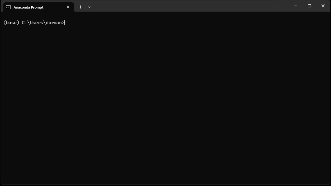
Fig. 9 The miniconda command line

Miniconda can thus be thought of as an extended version of the ordinary computer’s command line (“cmd”), where the Python program (python) and Python package management tool (conda) are pre-installed.

You can exit from the Miniconda command line by closing the window, or by typing exit and pressing Enter.

The Python command line

The first and simplest thing that the Miniconda command line provides, is the basic command-line interface to Python, i.e., the python program. The Python command line can be accessed by typing python in the Miniconda command line (see Using the Miniconda command line):

python

This opens the Python command line, which is marked by the >>> symbol.

Once inside the Python command line, Python expressions can be typed and executed by pressing Enter. For example, Fig. 10 shows what it looks like to open the Python command line and execute the two expressions, which define a list object (see Lists (list)) and print it:

a = [1,2,3]
print(a)

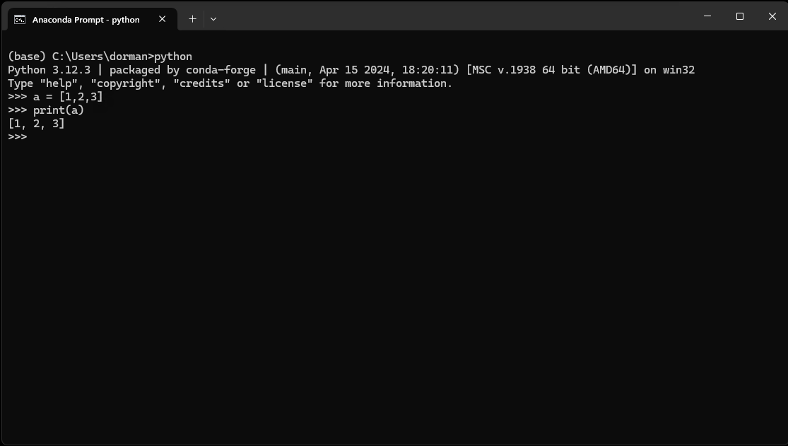
Fig. 10 Python interfaces: command line

The Python command line is convenient for experimenting with short and simple commands. When our code gets bigger and more complex, we usually prefer to keep it in persistent code files so that we can keep a record of our code, using Python script files (.py) (see Script files (.py)) or Jupyter notebooks (.ipynb) (see Jupyter Notebook).

To exit the Python command line, and return to the Miniconda command line, type exit() and press Enter:

exit()

Script files (.py)

A Python script is a plain text file, conventionally with the .py file extension. A .py file contains nothing but python code. For example, here is the contents of a python code file, such as a file named test.py, which contains two expressions, for creating and printing a list:

a = [1,2,3]
print(a)

A Python script can be created and edited using any plain text editor, whether a simple one such as Notepad++, or a specialized text editor for writing computer code such as Visual Studio Code (Fig. 11).

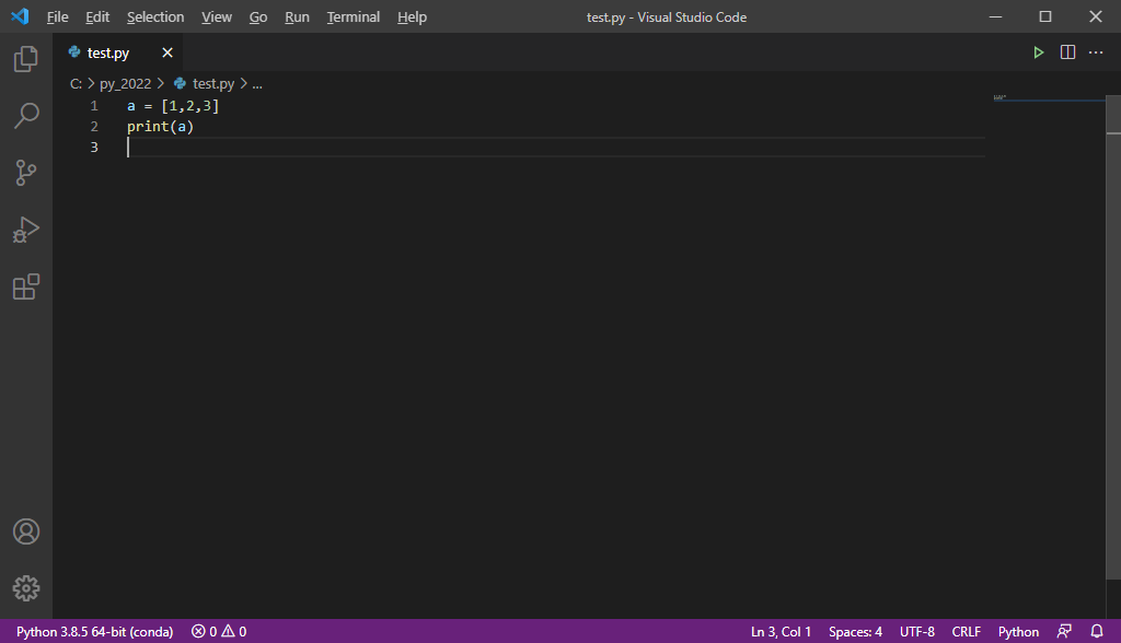
Fig. 11 Writing a Python script, a file named test.py

A python script can be executed in the command line, using an expression such as:

python test.py

where:

• python is the name of the Python command line program (The Python command line), and

• test.py is the filename (or file path) of a text file that contains the Python code to be executed.

As a result, the code is executed and any results are printed in the command line (Fig. 12).

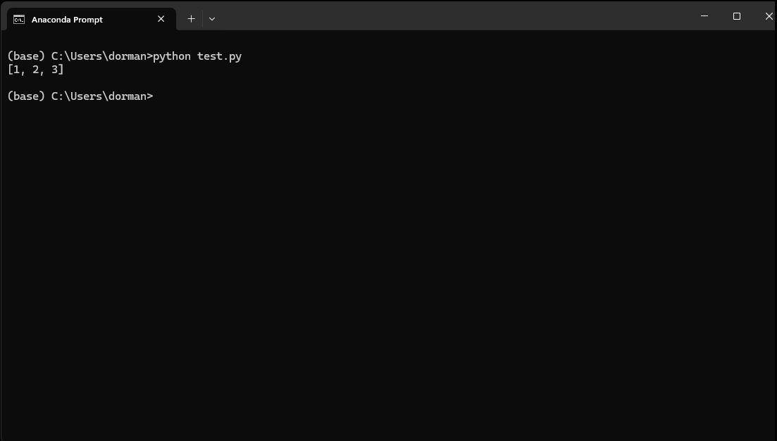
Fig. 12 Python interfaces: running a Python script file

IPython

IPython (“Interactive Python”) can be thought of as an enhanced Python command-line application, with many additional features. For example, IPython introduces new helper commands (such as ?, see Getting help), more sophisticated autocompletion, shortcuts for interacting with the operating system, and more (Fig. 13). Importantly, working with IPython involves a series of cells, with code input (marked with In) and output (marked with Out).

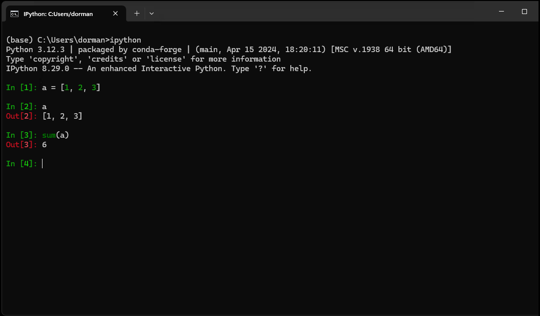
Fig. 13 Python interfaces: IPython

The IPython command line can be accessed by typing ipython in the Miniconda command line (see Using the Miniconda command line):

ipython

You can exit from IPython (and return to the Miniconda command line) by typing exit, or exit(), and pressing Enter:

exit

Jupyter Notebook

Jupyter Notebook is an extended interface of IPython, where, on top of the interactive interpreter and formatting, we also have a web interface to edit “notebooks” that permanently contain both the code and the output. Additionally, notebooks may contain formatted text, tables, images, equations, etc. (Fig. 14).

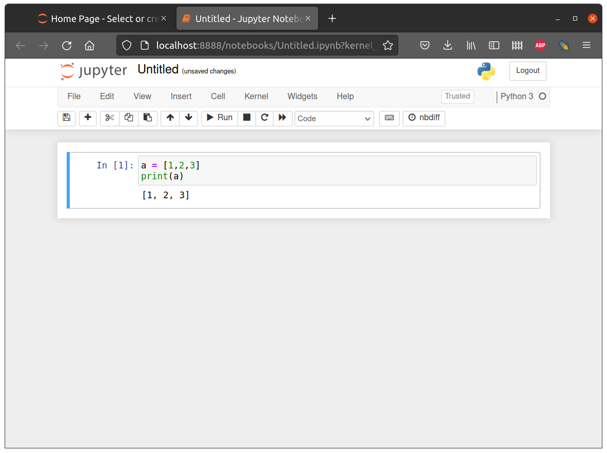
Fig. 14 Python interfaces: Jupyter notebooks

There are two “variants” of the jupyter notebooks interface (Table 5):

• The “classical” Jupyter Notebook interface

• The more recent and enhanced Jupyter Lab interface

Table 5 Jupyter interfaces

Interface	Command	Website
Jupyter Notebook	jupyter notebook	https://jupyter-notebook.readthedocs.io/en/stable/
Jupyter Lab	jupyter-lab	https://jupyterlab.readthedocs.io/en/latest/

In short, Jupyter Lab is a newer interface, extending the Jupyter Notebook functionality with new editing capabilities and utilities for working with Python. Jupyter Notebook are the older more focused interface, which includes just the “notebook” interface [1].

The Jupyter Notebook interface is a perfectly sufficient approach to run Python code for the purposes of this book, and in general. Therefore, in this chapter we demonstrate the Jupyter notebook interface. Note that these instructions are also applicable to Jupyter Lab, since it extends the Jupyter Notebook interface.

To use Jupyter Notebook, you need to install the notebook package, similarly to the way that any other Python package is installed. For example, when using Miniconda, the following expression may be used to install notebook:

conda install -c conda-forge notebook

However, do not run the above command just yet! We are going to elaborate on installing the required packages (including notebook) later on (see Installing packages). If you do not have Jupyter Lab installed (e.g., you are working on your laptop and installed Miniconda from scratch), then jump to the Installing packages section and follow the instructions to install the packages we will be working with in this book, including Jupyter Lab. When done, go back to this section to experiment with the notebook interface.

Note

The -c conda-forge part specifies that the “channel”, or package repository, for downloading the package named conda-forge will be used instead of the default. The conda-forge channel is a community-maintained channel which contains the newest versions of Python packages, and therefore is recommended. The default channel is maintained by the commercial company Anaconda, it does not necessarily contain the newest versions of packages, and is subject to paid license in some commercial settings, whereas conda-forge is completely free.

Note

Remember that installing Python packages with Miniconda, including Jupyter notebooks (the notebook package as shown above) or other packages (see Python packages), usually requires running the Miniconda command line as an administrator. This can be done (on Windows 10) by right-clicking on the Miniconda command line icon, then choosing Run as administrator.

To start the Jupyter Notebook interface, open the Miniconda command line, and navigate to the directory where your notebooks are stored (or where you would like to create a new notebook). Then, run jupyter notebook to start the Jupyter Notebook interface:

jupyter notebook

For example, if your working directory is C:\Users\dorman\Downloads, then you need to start the Miniconda command-line and run the following two expressions to open the Jupyter Notebook interface (for example, to create a new notebook):

cd C:\Users\dorman\Downloads
jupyter notebook

or the following expression to open an existing notebook named code_01.ipynb:

cd C:\Users\dorman\Downloads
jupyter notebook code_01.ipynb

Note

cd, one of the most useful commands in the command line, stands for “change directory”. Another useful command is dir, which prints directory contents. Try it out!

After running jupyter notebook, you should see some output printed in the console (Fig. 15). At the same time, the notebook interface should automatically open in the browser (Fig. 14).

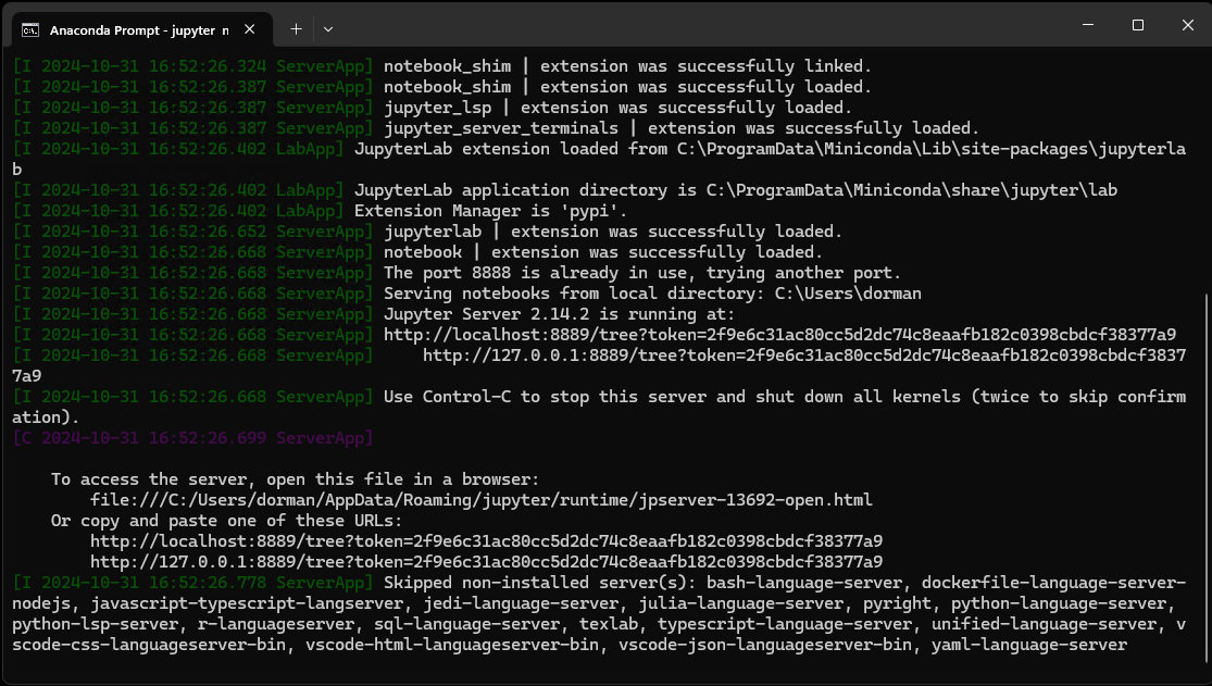
Fig. 15 Command line printout when running jupyter notebook

Jupyter notebooks are viewed and executed through a web browser, but they need to be connected to a running Python process. Therefore leave the console open as long as you are working with the Jupyter notebooks in the browser. When done, first close the Jupyter notebook tab(s) in the browser, and then terminate the jupyter notebook process with Ctrl+C.

Working with notebooks

Notebook files (.ipynb)

Notebooks are saved as .ipynb files (short for “IPython notebook”). .ipynb are plain text files, but more sophisticated ones then .py script files (see Script files (.py)). Importantly, .ipynb files contains not just Python code inputs, but also:

• the division into separate “cells” (see IPython),

• code outputs (see Code output), both textual and graphical ones, resulting from previous evaluations of the code cells (see Executing cells), if any, and

• non-code cells (see Cell types). (Do not worry if these terms are not clear yet—we are going to demonstrate them shortly.)

Accordingly, and unlike a plain .py script file, an .ipynb file does not make much sense when viewing and editing though a plain text editor. It is intended to be viewed and edited only through an interface that can process and display it, such as Jupyter Notebook.

A notebook documents the Python workflow, so that it can be kept for future reference or shared with other people.

To create a new notebook in the Jupyter Notebook interface:

• Click on the New button (in the top-right of the screen)

• From the dropdown menu, select Notebook; this opens another tab with the new notebook

• In the “Select Kernel” menu, select Python 3 (ipykernel)

By default, the newly created notebook will be named Untitled.ipynb. You can rename it through File→Rename… in the menu (or clicking on the file name, in the top ribbon). While working with the notebook, and before closing it, remember to save your progress using the File→Save Notebook, or by pressing Ctrl+S.

You can also open an existing notebook, by running jupyter notebook and then choosing it in the file browser, which displays all files in the directory where the jupyter notebook command was executed. Alternatively, you can open a particular notebook directly from the command line by specifying its name. For example, to open the notebook named code_01.ipynb in the current working directory run jupyter notebook code_01.ipynb.

Exercise 01-a

• Open the Miniconda command line.

• Navigate to your working directory, using a command such as cd C:\Users\dorman\Downloads.

• Start the Jupyter Notebook interface, using the jupyter notebook command.

• Create a new Jupyter Notebook.

• Rename the notebook to any name other than the default, such as code_01.ipynb.

• Save the notebook.

• Close the browser tab, then stop the Jupyter Notebook interface using Ctrl+C in the Miniconda command line.

• Re-open the notebook you just created, using a command such as jupyter notebook code_01.ipynb.

Cell types

Jupyter notebooks are composed of cells. There are two types of cells:

• Code cells

• Non-code cells, also known as Markdown cells

You can distinguish code cells by the square brackets displayed to the cell (i.e., [ ]), possibly filled with sequential IDs after the cells have been executed (i.e., [1], [2], etc.) (Fig. 14).

Code cells contain Python code, which can be executed, displaying the result (if any) immediately below the cell. We elaborate on code execution (Executing cells) and code output (Code output) below.

Markdown cells contain text, typically explanations, or background information, describing the code. Markdown cells follow the Markdown syntax, so in addition to plain text they may display headings, bold or italic text, bullet lists, tables, URLs, and so on. For example, the online version of the book you are reading right now is prepared from a set of Jupyter notebooks (one for each chapter), where all contents other than code are set using Markdown syntax. You can download the source .ipynb files (Fig. 17) to see how various elements, such as bullet lists, tables, etc., are specified.

Working modes

There are two “modes” when working inside a notebook:

• Navigation mode

• Cell editing mode

You can switch between the two modes as follows:

• When in the navigation mode, you can enter editing mode by pressing Enter. That way, you can edit the current cell.

• To exit editing mode, and return to navigation mode, press Esc.

When in navigation mode, there are quite a few things, related to cell organization, that you can do. The most common operations are summarized in Table 6.

Table 6 Common “navigation mode” operations in a Python notebook

Keyboard shortcut	Operation
↑ / ↓	Navigate between cells
A	Create new cell above current one
B	Create new cell below current one
D, D	Delete current cell
Y	Convert the current cell to a code cell
M	Convert the current cell to a markdown cell
C	“Copy” current cell
X	“Cut” current cell
V	“Paste” the copied or cut cell, below current cell

When in editing mode, you can type or edit cell contents, much like in a plain text editor. If the cell is a code cell, then the text is interpreted as Python code. If the cell is a markdown cell, then the text is interpreted as markdown text.

Executing cells

You can execute a cell by pressing Ctrl+Enter, or Shift+Enter. The difference between the two is that the latter advances to the next cell (Table 7). These keyboard shortcuts work in both editing and navigation modes.

• When executing a code cell, the code is sent to the underlying Python interpreter, and the result (if any) is displayed below the cell.

• When executing a markdown cell, the text is rendered, so that any formatting (such as bold text marked with **, as in **text**) is displayed

Table 7 Cell execution operations in a Python notebook

Keyboard shortcut	Operation
Ctrl+Enter	Execute current cell
Shift+Enter	Execute current cell & advance

Note that you can navigate between cells, skip cells, and execute the cells in a notebook, in any order you choose. The Python process in the background keeps track of the current state of the environment as a result of all code you have run so far. You can always reset the environment using the Kernel→Restart Kernel… button in the menu. In general, it makes sense to write the notebook assuming the cells will be executed in the given order. To run the entire notebook, from start to finish, you can use the Kernel→Restart Kernel and Run All Cells… button.

Exercise 01-b

• Create a Jupyter notebook and try the operations described above, as follows.

• Create two or more code cells, and two or more markdown cells

• Type some code into the code cells, and execute it using Ctrl+Enter. We have not learned any Python syntax yet. For now, you can insert the code expressions shown above to create and type a list (see The Python command line), or arithmetic expressions such as 10+5.

• Type text into the markdown cells and “execute” them too to display the text. (You can also check out markdown syntax rules online and use them to format your text.)

• Delete one of the cells by pressing the D key twice.

Code output

Code output appears below code cells, in case they have already been executed. It is important to understand that a Jupyter Notebook, in an .ipynb file, may store code as well as output. This is unlike a plain Python script, in a .py file (see Script files (.py)), which stores just Python code, withouth any output. Stored output can be confusing if you are not used to working with notebooks; for example, if you modify a code cell that already has “old” output, without re-running it, the revised code may no longer match the “old” output, up until you run it to calculate the “new” output. You can always remove all outputs from a notebook using the Kernel→Restart Kernel and Clear Output of All Cells… button. Alternatively, you can use the Kernel→Restart Kernel and Run All Cells… button to run the entire notebook from start to finish, thus calculating (or updating) all code outputs at once.

Usually, code output in a Jupyter notebook is just textual, in which case it is displayed in the notebook exactly the same way as it would appear in a Python command line (see The Python command line), or in an IPython command line (see IPython). However, since Jupyter notebooks are displayed in a web browser, they are able to dispay many other types of non-textual output that the command line cannot display. For example, Jupyter notebooks can display images, such as plots or maps (Fig. 19), which result from graphical Python functions.

Exporting

A Jupyter notebook can be exported into several formats, using the File→Save and Export Notebook As… menu. From there, choose the output format. For example, you can export a Jupyter notebook as:

• An HTML (.html) document, to place in a website

• A PDF (.pdf) document, to share with colleagues (requires xelatex, which is beyond the scope of this book)

• An Executable Script, i.e., a Python script (.py), to run in the command line (see Script files (.py))

Python packages

What are packages?

Packages are code collections that we can import in our Python script, or a Jupyter notebook, to make the functions defined there available to us.

The Python installation comes with numerous built-in packages, known as Python’s standard library. For example, the csv package, which provides basic methods for reading and writing CSV files, is part of the standard library (see Reading CSV files). Packages from the standard library, such as csv, do not need to be installed. However, they need to be loaded before use (see Loading packages).

There are many Python packages that are not part of the standard Python installation, known as third-party packages, or external packages. For example, pandas is a third-party Python package which has more advanced methods for reading CSV files than the csv package (see Reading from file). Since third-party packages are not part of the Python installation, they need to be installed in a separate step (see Installing packages). Once installed, third-party packages need to be loaded before use (see Loading packages), just like standard packages.

Installing packages

Python packages are installed using a package manager program. Two popular ones are conda (which comes with the Anaconda and Miniconda installations), and pip. When using Miniconda, Python packages can be installed from the Miniconda command line, using an expression such as:

conda install -c conda-forge PACKAGE

where the word PACKAGE needs to be replaced with the package name. For example, here is the specific expression that can be used to install the geopandas package:

conda install -c conda-forge geopandas

To run the examples in this book, you need to install several packages, most importantly geopandas and rasterio. Installing geopandas installs several dependencies that we are going to use, such as numpy, pandas and shapely. Other packages we are going to use, and need to be installed, include richdem and rasterstats. Overall, you need to install the following packages:

• notebook

• geopandas

• rasterio

• richdem

• rasterstats

You can install these packages using a single command, as follows:

conda install -c conda-forge notebook geopandas rasterio richdem rasterstats

A more standardized approach is to supply a text file with package specification (e.g., requirements.txt), listing the package names and (possibly) their specific versions. To install the packages that we are going to use in this book, navigate to the folder which contains the included requirements.txt file (see Table 3), then run the following command:

conda install -c conda-forge --file requirements.txt

As part of the installation you will see a printout of the package dependencies and versions that are going to be installed. Type y (yes) and press Enter to approve and proceed with the installation (Fig. 16).

As mentioned above, the Minoconda command line must be started as administrator when installing packages (see Jupyter Notebook).

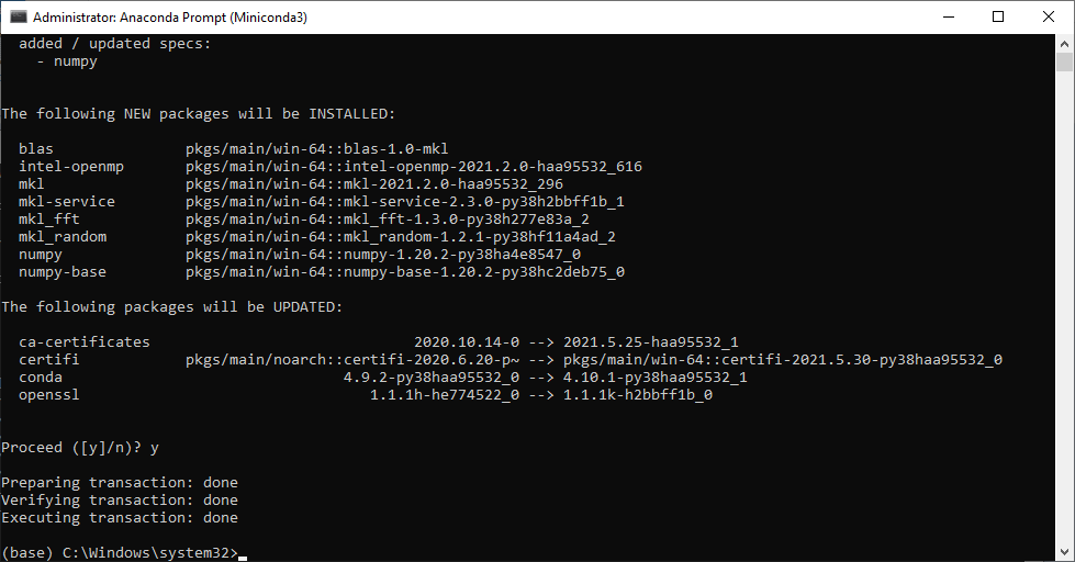
Fig. 16 Installing Python packages using conda install on the Miniconda command line

Note

When installing Python packages, it is considered best practice to work with environments. An environment can be thought of as an isolated space with a particular Python installation and a particular set of packages with specific versions. The user can create independent environments for different purposes. That way, any possible incompatibilities between Python packages are minimized. The concept of environments is beyond the scope of this book, but you can check out the basics in: https://docs.conda.io/projects/conda/en/latest/user-guide/getting-started.html#managing-environments.

Note

Installation of packages with conda can be quite slow. A faster alternative is mamba. To use it, first install mamba with conda install -c conda-forge mamba, then use it to install other packages, as in mamba install -c conda-forge geopandas.

Loading packages

A package can be loaded in two basic ways. In the first approach, we can import an entire package namespace, making all of the contents available in our script using import. For example, here is how we import the shapely package, which we are going to learn about in Geometries (shapely):

import shapely

Afterwards, we can access any function from the package, by typing shapely.FUNCTION. For example, shapely.Point is a function that creates a point geometry given x- and y-coordinates (which we learn about in shapely from type-specific functions):

shapely.Point((0, 1))

It is common practice to import a package under a different name which is shorter to type, using the import package as name expression. For example, if we import the shapely package under the name s:

import shapely as s

We can now access all of the functions in shapely using s.*, instead of shapely.*:

s.Point((0, 1))

In the second approach, we can import just a particular function, using from and import:

from shapely import Point

After that, we can refer to the particular function(s) we imported by their name alone, as in:

Point((0, 1))

We can also import several functions at once, separated by commas:

from shapely import Point, Polygon

and we can import functions under a different name:

from shapely import Point as pnt, Polygon as pol

The advantage of importing specific function(s) from a package, as opposed to importing an entire package, is that the code is concise, and that it is evident from the beginning which specific functions the code uses. The disadvantage is that we can only use the specific function we imported, and not any other functions from the package. In this book we will use the first approach of importing entire packages, because:

• we will be using many different functions from each package throughout the examples, and

• to make it clear which package each new function we learn about comes from.

File paths

At first, the simple Python scripts we are going to write will be self-contained, in the sense that the data they operate on are created as part of the script itself, and the results are not saved to permanent storage (e.g., on the hard disk). However, in realistic data analysis it is often necessary to:

• import existing data from disk at the beginning of the script, and to

• export the results to a file on disk at the end.

For example, a script that transforms a CSV file with lon/lat columns into a point Shapefile (see below) will be composed of the following parts:

• Import the CSV file (see Reading from file)

• Transform the table to a point layer (see Table to point layer)

• Export the point layer to a Shapefile (see Writing GeoDataFrame to file)

import pandas as pd
import geopandas as gpd
dat = pd.read_csv('data/world_cities.csv')  ## Import CSV file
geom = gpd.points_from_xy(dat['lon'], dat['lat'])
geom = gpd.GeoSeries(geom)
dat = gpd.GeoDataFrame(dat, geometry=geom, crs=4326)
dat.to_file('output/world_cities.shp')      ## Export Shapefile

Exercise 01-c

• What is the purpose of the first two expressions in the above code section? Explain what they do.

Do not worry about the functions and methods used in the code, as we are going to cover them in detail throughout the following chapters. For now, pay attention just to the the file paths:

• 'data/world_cities.csv'—Path to the CSV file to import

• 'output/world.cities.shp'—Path of the Shapefile to export

In general, when reading or writing a file in a Python script, we need to refer to the file location, or the file path. There are two basic ways to specify a file path:

• An absolute path, such as 'C:/Users/dorman/Downloads/data/world_cities.csv'

• A relative path, such as 'data/world_cities.csv' or 'world_cities.csv'

Note that, in Python code, unlike in the Miniconda command line (see Using the Miniconda command line), you must use /, and not \ when writing file paths!

Note

In this book, we specify file paths using a string with path components separated by /. This is the simplest method, and it is sufficient for our needs. The best practice, however, is to use the pathlib standard package, which has many more feaures for handling and manipulating paths. For more details, see the documentation.

In an absolute path, we specify the complete path starting from the file system “root” and up to the file location. On Windows, this means we start from the drive specification (such as 'C:/'), then specify any directories and sub-directories, separated by /, and finally the file name. For example, the absolute file path 'C:/Users/dorman/Downloads/data/world_cities.csv' means that we refer to:

• the file named world_cities.csv,

• which is located in the data directory,

• which is located in the Downloads directory,

• which is located in the dorman directory,

• which is located in the Users directory,

• which is located in drive C:.

In a relative path, we specify a partial path that begins with the script, or notebook, location. For example, the relative path 'data/world_cities.csv' means that we refer to:

• the file named 'world_cities.csv',

• which is located in the 'data' directory,

• which is located in the directory where our notebook or script is.

Specifying the just a file name, such as 'world_cities.csv' is a special case of a relative path, meaning that the file is located in the same directory where our script is.

When writing code, relative path are usually preferred, because they are more general. For example, when sending a script along with a data directory where the data are to a colleague, a relative file path such as 'data/world_cities.csv' will work regardless of the directory name where the colleague saved the script and data directory, as long as they are “together”. However, when a script contains an absolute file path, such 'C:/Users/dorman/Downloads/data/world_cities.csv', it is much less likely to work as-is, unless the colleague saves the file world_cities.csv in exactly the same location as specified in the script.

In agreement with the recommendation, in all code samples in this book, we are going to use relative file paths starting with data, such as 'data/world_cities.csv'. To reproduce the examples in the book, you can:

• Download the sample data files (see Sample data) and save them in a sub-directory named data

• Download the .ipynb notebook file of any particular chapter, using the “download” button (in the top-left of the web page) and choosing the .ipynb option (Fig. 17) into the “main” directory

• Open the notebook in the Jypyter Notebook interface (see Jupyter Notebook)

Of course you can use any other location for the data, but then you also need to change the file paths, accordingly.

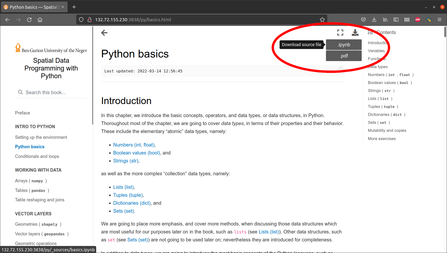
Fig. 17 Button to download the .ipynb source of a book chapter

Code comments

Code comments in Python are marked with #. Anything to the right of the # symbol is ignored by the interpreter. Code comments are usually used to describe the intention in an entire code section:

# List of selected numbers
a = [1,2,3]
print(a)

[1, 2, 3]

or in specific expressions:

a = [1,2,3]  # List of selected numbers
print(a)

[1, 2, 3]

Code comments should optimally provide useful information which is not evident from the code itself. For example, this is a useful code comment:

d = 5  # Distance in km

while this one is not very useful:

d = 5  # Assign 5 to 'x'

Getting help

When learning a new programming language, one of the most important skills is finding answers to questions. Accordingly, when reading this book keep in mind that the purpose is to become familiar with the general principles and workflow types involving spatial data in Python. There is no need to memorize the material, because once you are familiar with the fundamentals you will be able to formulate the right question to search online (e.g., in Google).

Some quick questions can be answered offline, using Pythons’ built-in help methods. For example, you can get a concise summary of any built-in function, or any other object, using Pythons’ built-in help function:

help(len)

Help on built-in function len in module builtins:

len(obj, /)
    Return the number of items in a container.

There is an alternative, IPython-specific, method, to get help, using an expression of the form function?. i.e., a function name followed by ?. For example, try running range? in a Jupyter notebook to see the help text for the range function (see The range function).

It should be noted that built-in help pages tend to be concise and use many technical terms, which can be difficult for beginners. It is often more helpful to search the function name on Google to view more user-friendly resources, such as online tutorials (Fig. 18).

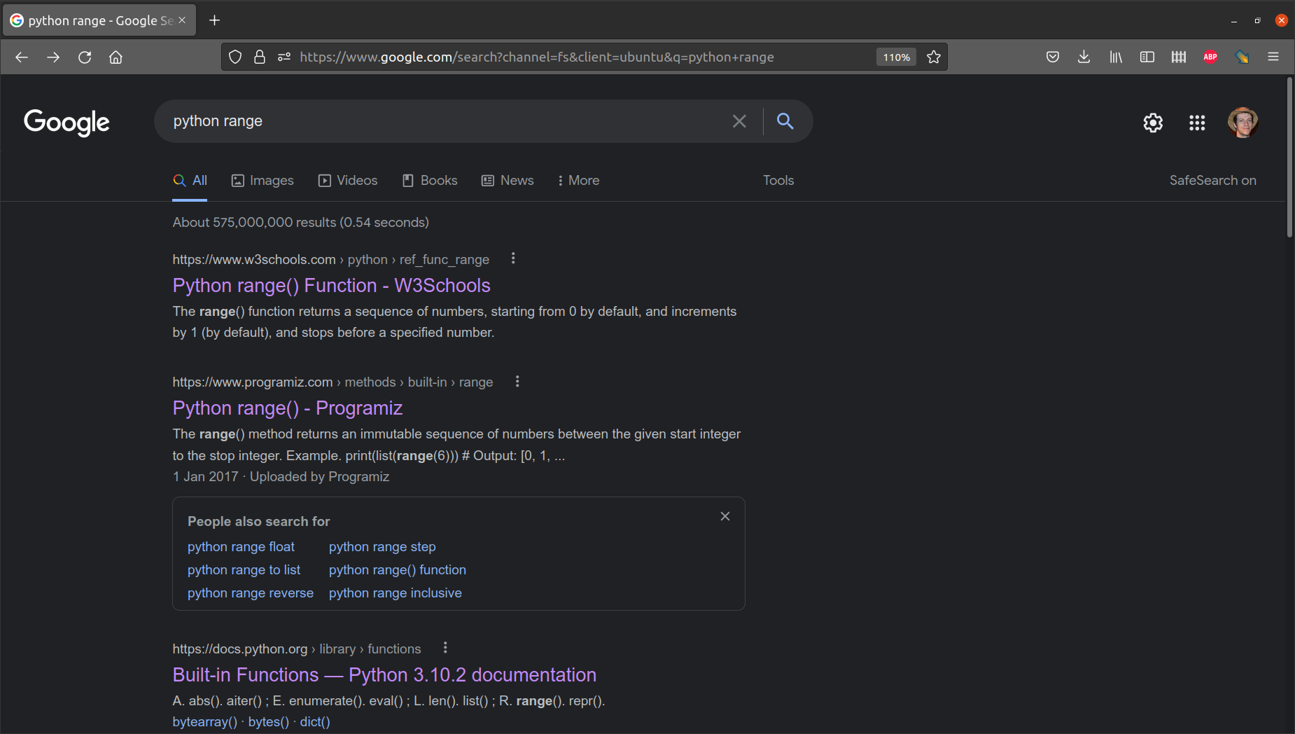
Fig. 18 Results for search term “python range” on https://www.google.com/

More exercises

Exercise 01-d

• Start the Jupyter Notebook interface according to the instructions above.

• Create a new notebook.

• Create a new cell with the code shown below.

• Execute the cell. You should see the output [1,2,3] below it.

a = [1,2,3]
print(a)

Exercise 01-e

• Create a cell and with the code shown below. This code section uses the numpy package to create an array object (see Arrays (numpy)).

• Execute the cell. You should see an array object printout.

import numpy as np
b = np.array([[1,2,3],[4,5,6],[7,8,9],[10,11,12]])
b

Exercise 01-f

• Download the Sample data.

• Place the data in a sub-directory named data inside the directory where your Jupyter notebook is.

• Create another cell with the code shown below (Fig. 19). This code section imports a vector layer from a Shapefile named 'muni_il.shp', and then plots it.

• You should see a plot as shown in Fig. 20.

import geopandas as gpd
towns = gpd.read_file('data/muni_il.shp')
towns.plot();

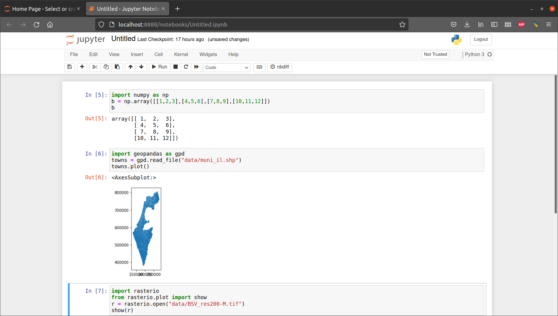
Fig. 19 geopandas map example in a Jupyter notebook

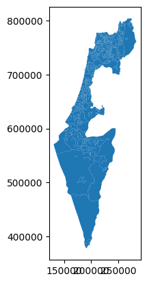
Fig. 20 Solution of exercise-01-f: Map of muni_il.shp vector layer

Exercise 01-g

• Create another cell with the code shown below. This code section imports a raster from a file named 'BSV_res200-M.tif', and then plots it.

• You should see a plot as shown in Fig. 21.

import rasterio
import rasterio.plot
r = rasterio.open('data/BSV_res200-M.tif')
rasterio.plot.show(r);

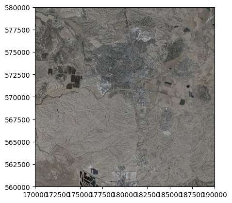
Fig. 21 Solution of exercise-01-g: Image of BSV_res200-M.tif raster

---

[1]

See https://stackoverflow.com/questions/50982686/what-is-the-difference-between-jupyter-notebook-and-jupyterlab for more information about the difference between Jupyter Notebook and Jupyter Lab.