Geometries (shapely)

Last updated: 2024-12-15 18:10:24

---

Introduction

In the previous chapters we covered the basics of working with Python, starting with the working environment setup (see Setting up the environment) to advanced methods of working with tables (Table reshaping and joins). Now, we move on to the main topic of this book, working with spatial data.

Spatial data can be divided into two categories:

• Vector layers—points, lines, and polygons, associated with attributes

• Rasters—numeric arrays representing a regular grid over a rectangular area

In the next three chapters, we go through the basics of working with the first type, vector layers, in Python. In this chapter, we cover the shapely package, which is used to represent and work with individual vector geometries. The next two chapters (see Vector layers (geopandas) and Geometric operations) deal with another package, called geopandas, which is used to represent and work with vector layers. The individual geometries within a vector layer are stored as shapely geometries. Therefore it is essential to be familiar with the shapely package, first, before moving on geopandas.

Specifically, in this chapter we are going to cover the following topics:

• Creating geometry objects (see Creating geometries)

• Extracting geometry properties, such as:

  • Geometry type (see Geometry type)

  • Coordinates (see Geometry coordinates)

  • Derived properties, such as length and area (see Derived properties)

• Deriving new geometries, from:

  • Individual geometries (see New geometries 1 (shapely)), e.g., calculating geometry centroid

  • Pairs of geometries (see New geometries 2 (shapely)), e.g., calculating the intersection (i.e., shared area) of two geometries

• Evaluating boolean relations between geometries (see Boolean methods (shapely)), e.g., whether one geometry intersects with another or not

• Calculating distances (see Distance (shapely))

• Transforming points to a line (see Points to line (shapely))

What is shapely?

shapely is a Python package for working with vector geometries, that is, the geometric component of vector layers (the other component being non-spatial attributes). shapely includes functions for creating geometries, as well as functions for applying geometric operations on geometries, such as calculating the centroid of a polygon.

Technically, shapely is a Python interface to the Geometry Engine Open Source (GEOS) software. GEOS is used in numerous open-source programs other than shapely, such as QGIS, and interfaced in many programming languages, such as the sf package in R.

By design, shapely only deals with individual geometries, their creation, their derived properties, and spatial operation applied to them. shapely does not support reading or writing geometries to vector layer file formats (e.g., Shapefile), or more complex data structures to represent collections of geometries with or without non-spatial attributes (i.e., vector layers). These are accomlished with geopandas, which builds on top of pandas, shapely (Fig. 5), and other packages, to provide high-level methods to work with complete vector layers.

Note

The shapely documentation (Fig. 37) is quite detailed, and has many illustrations which are useful to understand how the various functions work.

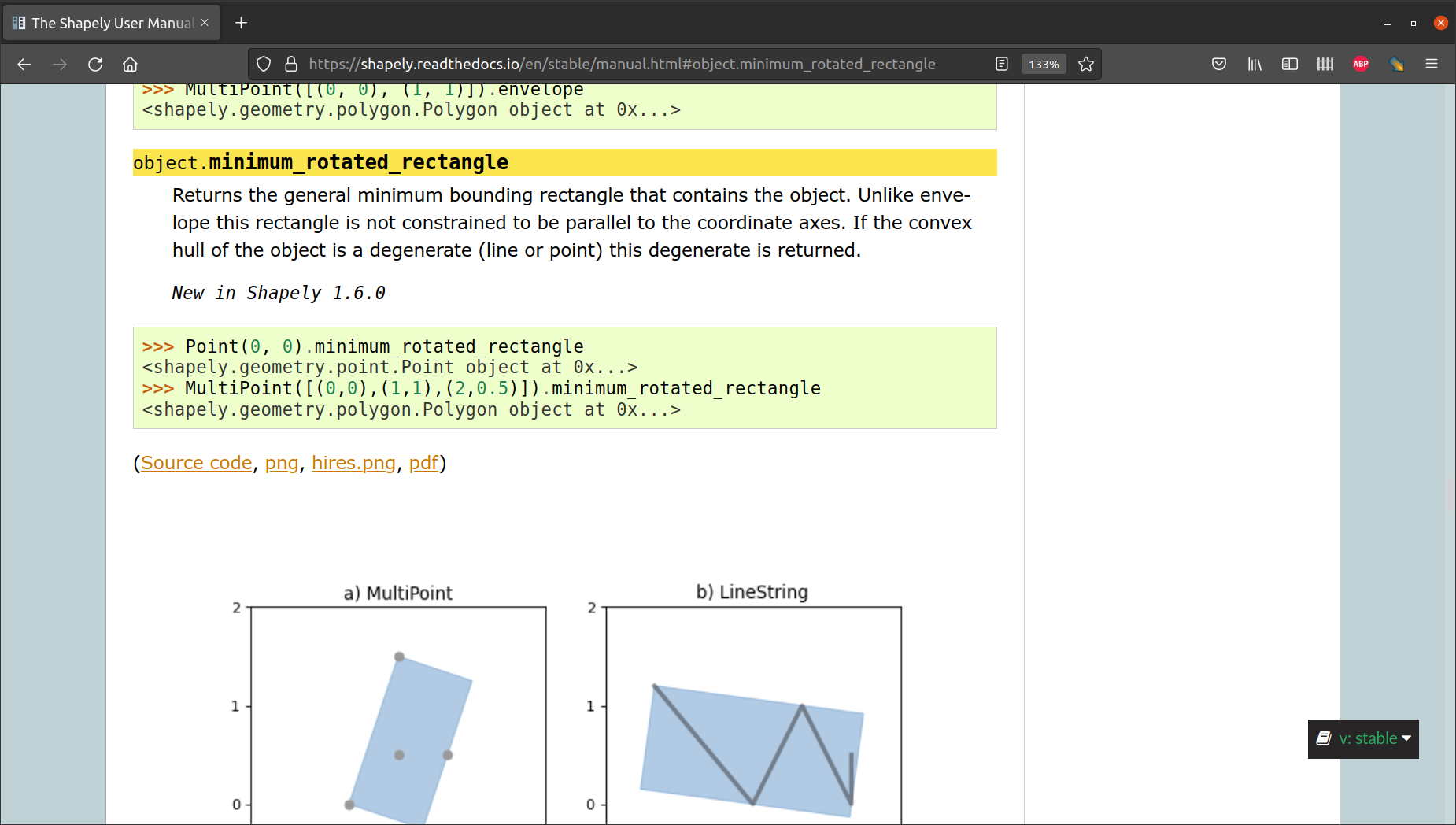
Fig. 37 The Shapely User Manual

What are Simple Features?

The GEOS software, and accordingly also the shapely package, implements the Simple Features specification of geometry types. The geometry type specification and functions may be familiar to you, since both the GEOS software and the Simple Features standard are widely used in open-source GIS software and in other programming languages, such as R’s sf package and the PostGIS spatial database.

The Simple Features specification defines at least 17 geometry types, but only seven types are commonly used in spatial analysis. These are shown in Fig. 38. Note that there are separate geometry types for points ('Point'), lines ('LineString'), and polygons ('Polygon'), as well are their multi-part versions ('MultiPoint', 'MultiLineString', 'MultiPolygon'), which sums up to the first six geometry types. The multi-part versions are intended for geometries that contain more than one single-part geometry at once. The seventh type ('GeometryCollection') is intended for any combination of the other six types.

Fig. 38 Simple Feature geometry types

Well Known Text (WKT) is a plain text format for representing Simple Feature geometries, and part of the Simple Feature standard. WKT is understood by many programs, including shapely, the sf package in R, and PostGIS. WKT strings of the geometries shown in Fig. 38 are given in Table 16 [1].

Table 16 Simple feature geometry types and WKT examples

Type	WKT example
'Point'	POINT (30 10)
'LineString'	LINESTRING (30 10, 10 30, 40 40)
'Polygon'	POLYGON ((35 10, 45 45, 15 40, 10 20, 35 10),(20 30, 35 35, 30 20, 20 30))
'MultiPoint'	MULTIPOINT (10 40, 40 30, 20 20, 30 10)
'MultiLineString'	MULTILINESTRING ((10 10, 20 20, 10 40),(40 40, 30 30, 40 20, 30 10))
'MultiPolygon'	MULTIPOLYGON (((40 40, 20 45, 45 30, 40 40)),((20 35, 10 30, 10 10, 30 5, 45 20, 20 35),(30 20, 20 15, 20 25, 30 20)))
'GeometryCollection'	GEOMETRYCOLLECTION (POINT (40 10),LINESTRING (10 10, 20 20, 10 40),POLYGON ((40 40, 20 45, 45 30, 40 40)))

Don’t worry if you are not familiar with the exact syntax of the WKT format. You will have an opportunity to see various WKT strings in the examples in this chapter. For now, just note that these are strings specifying the geometry type and the coordinates comprising the geometry. Parentheses (() are used the indicate the nested structure of coordinate sequences within the geometry, such as the separate polygons comprising a 'MultiPolygon' geometry, or the exterior and interior (i.e., holes) in a 'Polygon'. For example:

• POINT (30 10)—A point at (30,10)

• LINESTRING (0 0, 0 1)—A straight line going from (0,0) to (0,1)

Creating geometries

shapely from WKT

Before starting to work with shapely, we need to load the package:

import shapely

One way to create a shapely geometry object is to import a WKT string. To convert a WKT string into a shapely geometry, we pass the WKT string to the shapely.from_wkt function. In our first example, we create a polygon named pol1. Note that this is a rectange, composed of five coordinates. The fifth coordinate is identical to the first, used to “close” the shape, as required by the Simple Features standard:

pol1 = shapely.from_wkt('POLYGON ((0 0, 0 -1, 7.5 -1, 7.5 0, 0 0))')

Typing a shapely geometry in a Jupyter notebook conveniently draws a small figure:

pol1

We can also print the geometry, which prints its WKT string representation:

print(pol1)

POLYGON ((0 0, 0 -1, 7.5 -1, 7.5 0, 0 0))

The type of a shapely geometry consists of several components, starting from the general class, shapely.geometry, and ending with the specific geometry type, such as 'Polygon':

type(pol1)

shapely.geometry.polygon.Polygon

Let us create another polygon geometry, named pol2:

pol2 = shapely.from_wkt('POLYGON ((0 1, 1 0, 2 0.5, 3 0, 4 0, 5 0.5, 6 -0.5, 7 -0.5, 7 1, 0 1))')
print(pol2)

POLYGON ((0 1, 1 0, 2 0.5, 3 0, 4 0, 5 0.5, 6 -0.5, 7 -0.5, 7 1, 0 1))

This time we have more coordinates, and, accordingly, the shape of the polygon is more complex:

pol2

Finally, let us create another type of geometry, a 'MultiPolygon', named pol3. Note how the 'MultiPolygon' has several sequences of shapes, representing the outline and hole(s) of one or more polygons:

pol3 = shapely.from_wkt('''
MULTIPOLYGON
(((40 40, 20 45, 45 30, 40 40)),
((20 35, 10 30, 10 10, 30 5, 45 20, 20 35), (30 20, 20 15, 20 25, 30 20)))
''')

Note

The above expression uses multi-line string input in Python, using the ''' (or ''') character at the start and end of the string. This tells the Python interpreter that the string spans several lines. Otherwise we would get an error since a “newline” character ends the expression.

In pol3, we have one polygon without any holes, and another polygon that has one hole:

pol3

Exercise 07-a

• Go to the WKT article on Wikipedia.

• Locate examples of other types of geometries, such as 'Point', 'LineString', 'MultiPoint', and 'MultiLineString'. Create the corresponding shapely geometries.

• Print the shapes to inspect them graphically. Compare to the figures on Wikipedia.

shapely from type-specific functions

Another method of creating shapely geometries is to pass lists of coordinates, or lists of geometries, to specific functions. The required argument is different in the various functions, according to the geometry type (Table 17), as shown in the examples below.

Table 17 shapely functions to create geometries

Function	Geometry type
shapely.Point	'Point'
shapely.MultiPoint	'MultiPoint'
shapely.LineString	'LineString'
shapely.MultiLineString	'MultiLineString'
shapely.Polygon	'Polygon'
shapely.MultiPolygon	'MultiPolygon'
shapely.GeometryCollection	'GeometryCollection'

For example, shapely.Point is the simplest function to create a shapely geometry. It creates a 'Point' geometry, accepting a tuple of the form (x,y) with the point coordinates:

pnt1 = shapely.Point((2, 0.5))
pnt1

A 'MultiPoint', however, is created from a list of tuples, where each list element represents an individual point, using shapely.MultiPoint:

pnt2 = shapely.MultiPoint([(2, 0.5), (1, 1), (-1, 0), (1, 0)])
pnt2

A 'LineString' is also created from a list of tuples, using shapely.LineString:

line1 = shapely.LineString([(2, 0.5), (1, 1), (-1, 0), (1, 0)])
line1

A 'MultiLineString' can be created from a list of 'LineString' geometries, using shapely.MultiLineString:

l1 = shapely.LineString([(2, 0.5), (1, 1), (-1, 0), (1, -1)])
l2 = shapely.LineString([(-2, 1), (2, -0.5), (3, 1)])
line2 = shapely.MultiLineString([l1, l2])
line2

Exercise 07-b

• The shapely.GeometryCollection function accepts a list of geometries, and returns a 'GeometryCollection' composed of them.

• Use the above objects to construct and plot a 'GeometryCollection' that contains a point, a line, and a polygon.

A 'Polygon' can be created using the shapely.Polygon function and using a coordinate sequence where the first and last points are identical:

shapely.Polygon([(0, 0), (0, -1), (7.5, -1), [7.5, 0], (0, 0)])

Optionally, a second list may used to pass sequence(s) comprising polygon holes. For example, the following modified expressions create a polygon with one hole:

coords_exterior = [(0, 0), (0, -1), (7.5, -1), [7.5, 0], (0, 0)]
coords_interiors = [[(0.4, -0.3), (5, -0.3), (5, -0.7), (0.4, -0.7), (0.4, -0.7)]]
shapely.Polygon(coords_exterior, coords_interiors)

A 'MultiPolygon' can be created from a list of individual 'Polygon' geometries, using shapely.MultiPolygon:

shapely.MultiPolygon([pol1, pol2])

Note that what we got in the last expression is an individual 'MultiPolygon' geometry, not two separate polygon geometries:

print(shapely.MultiPolygon([pol1, pol2]))

MULTIPOLYGON (((0 0, 0 -1, 7.5 -1, 7.5 0, 0 0)), ((0 1, 1 0, 2 0.5, 3 0, 4 0, 5 0.5, 6 -0.5, 7 -0.5, 7 1, 0 1)))

Note

The above 'MultiPolygon' geometry is considered invalid, i.e., not in agreement with the Simple Features specification of 'Polygon'/'MultiPolygon' “validity”. Validity can be examined using the .is_valid property. It is also suggested by the green/red color of the geometry visualization. Specifically, a valid 'MultiPolygon' geometry cannot overlap in an infinite number of points.

shapely from GeoJSON-like dict

Our third method to create shapely geometries is the shapely.geometry.shape function. This function accepts a GeoJSON-like dict with the geometry definition. In general, the dict needs to have two properties:

• The 'type' property contains the geometry type

• The 'coordinates' property contains the sequences of geometries/parts/coordinates, as lists or tuples

For example, the following expression uses shapely.geometry.shape to create a 'Point' geometry:

shapely.geometry.shape({'type': 'Point', 'coordinates': (0, 1)})

The following expression uses shapely.geometry.shape to create a 'MultiPolygon' geometry. Accordingly, the input dict is more complex:

d = {
  'type': 'MultiPolygon',
  'coordinates': [
    [
      [[40, 40], [20, 45], [45, 30], [40, 40]]
    ],
    [
      [[20, 35], [10, 30], [10, 10], [30, 5], [45, 20], 
      [20, 35]], 
      [[30, 20], [20, 15], [20, 25], [30, 20]]
    ]
  ]
}
shapely.geometry.shape(d)

Geometry type

As evident in all of the above examples, the information contained in a shapely geometry is basically a pair of items:

• The geometry type definition, such as 'Point'

• The coordinate sequence(s) of all shapes comprising the geometry, such as (0,1)

(The exception being 'GeometryCollection', where the second item is a collection of geometries, not coordinates.)

Using shapely methods, we can access these two items. In this section we show how to access the geometry type, which is straightforward. In the next section, we discuss the methods to access the coordinates, which is more complex (see Geometry coordinates).

The .geom_type property of a shapely geometry contains the geometry type:

pol1.geom_type

'Polygon'

Note that the .geom_type is a string:

type(pol1.geom_type)

str

Geometry coordinates

Overview

The other component of a geometry (in addition to geometry type, see Geometry type) is the coordinates. In the following sub-sections, we demonstrate the ways we can access the coordinates of the five most commonly used geometry types (Table 18).

Table 18 Accessing shapely geometry coordinates

Geometry type	Access method
Point coordinates	.coords
LineString coordinates	.coords
MultiLineString coordinates	.geoms[0].coords
Polygon coordinates	.exterior.coords, .interiors[0].coords
MultiPolygon coordinates	.geoms[0].exterior.coords, .geoms[0].interiors[0].coords

As we will see, the access method is specific per geometry types, due to their different levels of complexity.

In practice, it is rarely necessary to access the coordinates directly, because there are predefined functions for all common operations involving the coordinates (such as calculating the centroid, see Centroids (shapely)). However, being aware of the coordinate access methods gives you the freedom, if necessary, to develop any type of geometric calculation or algorithm, even if it is not defined in shapely, or any other software. Additionally, through the access methods we will become more familiar with the structures of the various geometry types.

Point coordinates

'Point' geometry coordiantes are accessible thought the .coords property. The returned object is of a special type called CoordinateSequence:

pnt1.coords

<shapely.coords.CoordinateSequence at 0x76b3581dff80>

It can be converted to a more convenient form, of a list, using the list function:

list(pnt1.coords)

[(2.0, 0.5)]

As we can see, coordinates are organized as a list of tuples. In this case, since with are talking about a Point geometry, the list is of length 1, containing a tuple of the point coordinates.

LineString coordinates

The coordinates of a 'LineString' are accessible in exactly the same way as those of 'Point' (see Point coordinates).

list(line1.coords)

[(2.0, 0.5), (1.0, 1.0), (-1.0, 0.0), (1.0, 0.0)]

However, the list is not of length 1, but at least of length 2. For line1, the list is of lenght 4, because the line is composed of four points.

MultiLineString coordinates

For 'MultiLineString' geometries, there is no direct .coords method to access the coordinates of all parts at once. Instead, the parts have to be accessed one by one, using the .geoms property, combined with an index (starting from 0). Any particular “part” of a 'MultiLineString' geometry behaves the same way as a 'LineString' geometry. Once we are “inside” a particular 'MultiLineString' part, we can use any of the properties or methods applicable to a 'LineString' geometry, such as coords.

For example, consider the 'MultiLineString' named line2:

line2

Here is how we can access its two parts:

line2.geoms[0]

line2.geoms[1]

Note that each part of a 'MultiLineString' is a 'LineString':

type(line2.geoms[0])

shapely.geometry.linestring.LineString

In case we do not know in advance how many parts there are, we can use the len function to find out:

len(line2.geoms)

2

Going further, we can access the coordinates of each part using .coords (see LineString coordinates):

list(line2.geoms[0].coords)

[(2.0, 0.5), (1.0, 1.0), (-1.0, 0.0), (1.0, -1.0)]

list(line2.geoms[1].coords)

[(-2.0, 1.0), (2.0, -0.5), (3.0, 1.0)]

Polygon coordinates

'Polygon' coordinate sequences are associated with the concepts of exterior and interiors coordinate sequences:

• The exterior is the outer bound of the polygon. There is only one exterior sequence per polygon. The .exterior property gives direct access to the exterior geometry.

• The interiors refers to polygon holes. There can be zero or more holes in each polygon. Accordingly, the .interiors property is a sequence of length zero or more.

For example, pol1 is a 'Polygon' with no holes:

pol1

We can access its exterior coordinates using .exterior:

pol1.exterior

followed by .coords

list(pol1.exterior.coords)

[(0.0, 0.0), (0.0, -1.0), (7.5, -1.0), (7.5, 0.0), (0.0, 0.0)]

The interior sequence(s), if any, can be accessed through .interiors; in this case, the interiors sequence is empty:

len(pol1.interiors)

0

You will get a chance to see a non-empty .interiors sequence in the next example (see MultiPolygon coordinates).

MultiPolygon coordinates

'MultiPolygon' coordinates are accessed by first extracting one of the polygon parts, using .geoms, similarly to the way we extract 'MultiLineString' parts (see MultiLineString coordinates). Each of the 'MultiPolygon' parts is a 'Polygon' geometry. Therefore, we can use the exterior and interiors methods to get the coordinates of each part, just like with a standalone 'Polygon' (see Polygon coordinates).

For example, pol3 is a 'MultiPolygon' geometry with two parts, where one of the parts has one hole:

pol3

The .geoms method lets us access the parts one by one:

pol3.geoms[0]

pol3.geoms[1]

Note that each part of a 'MultiPolygon' geometry is a 'Polygon' geometry:

type(pol3.geoms[0])

shapely.geometry.polygon.Polygon

Starting with the first part, here is the exterior:

pol3.geoms[0].exterior

list(pol3.geoms[0].exterior.coords)

[(40.0, 40.0), (20.0, 45.0), (45.0, 30.0), (40.0, 40.0)]

As expected, there are no interiors:

len(pol3.geoms[0].interiors)

0

Now, here is the second part of the 'MultiPolygon':

pol3.geoms[1]

Here is the exterior:

pol3.geoms[1].exterior

and its coordinates:

list(pol3.geoms[1].exterior.coords)

[(20.0, 35.0),
 (10.0, 30.0),
 (10.0, 10.0),
 (30.0, 5.0),
 (45.0, 20.0),
 (20.0, 35.0)]

This part does contain interiors, specifically one “interior” (i.e., hole):

len(pol3.geoms[1].interiors)

1

Here is how we can access the first (and only) interior:

pol3.geoms[1].interiors[0]

and its coordinates:

list(pol3.geoms[1].interiors[0].coords)

[(30.0, 20.0), (20.0, 15.0), (20.0, 25.0), (30.0, 20.0)]

Derived properties

Overview

The geometry type (Geometry type), and the geometry coordinates along with their division to parts and interior/exterior sequences (Geometry coordinates), are basic “internal” geometry properties. Additionally, there are derived useful properties that can be calculated for each geometry.

In the next few section we cover several useful derived geometry properties (Table 19).

Table 19 shapely geometry derived properties

Property	Meaning
.bounds	Bounds (shapely)
.length	Length (shapely)
.area	Area (shapely)

Bounds (shapely)

The .bounds property of a shapely geometry contains its bounds, i.e., the coordinates of the bottom-left \((x_{min}, y_{min})\) and top-right \((x_{max}, y_{max})\) corner of its bounding box. The four coordinates are returned in the form of a tuple of length four \((x_{min}, y_{min}, x_{max}, y_{max})\). For example:

pol1.bounds

(0.0, -1.0, 7.5, 0.0)

pol2.bounds

(0.0, -0.5, 7.0, 1.0)

pol3.bounds

(10.0, 5.0, 45.0, 45.0)

Note that even a 'Point' geometry has bounds, where \(x_{min}\) is equal to \(x_{max}\), and \(y_{min}\) is equal to \(y_{max}\):

pnt1.bounds

(2.0, 0.5, 2.0, 0.5)

The shapely.box function can be used to create a 'Polygon' geometry reflecting the bounding box. For example, the following expression creates the bounding box geometry of pol3:

shapely.box(*pol3.bounds)

Note that the shapely.box function requires four separate positional arguments (i.e., xmin,ymin,xmax,ymax), rather than a tuple. Therefore, in the last expression, we used the positional argument technique (see Variable-length positional arguments) to “unpack” the pol3.bounds tuple into four arguments passed to box. The equivalent expression without using the positional argument technique would be:

shapely.box(pol3.bounds[0], pol3.bounds[1], pol3.bounds[2], pol3.bounds[3])

Note

The .envelope property (Table 20) can be used to directly access the bounding box geometry.

Length (shapely)

The .length property gives the length of the geometry. For example, here we calculate the length of line1, a 'LineString' geometry:

line1

line1.length

5.354101966249685

and here we calculate the length of line2, which is a 'MultiLineString' geometry:

line2

line2.length

11.664947454140234

Note that the length (or area, see Area (shapely)) of a multi-part geometry is the sum of lengths (or areas) of all its parts. For example, using the access methods shown above (see Geometry coordinates), we can calculate the length of the two parts that comprise the 'MultiLineString' named line2:

line2.geoms[0].length

5.5901699437494745

line2.geoms[1].length

6.07477751039076

and demonstrate that the sum of lengths of the two parts is equal to the total geometry length:

line2.geoms[0].length + line2.geoms[1].length == line2.length

True

Keep in mind that:

• The .length of 'Point' or 'MultiPoint' geometries is equal to 0

• The .length of 'Polygon' or 'MultiPolygon' geometries refers to the summed perimeters of the exterior and all interiors

Exercise 07-c

• pol1 is a 'Polygon' geometry representing a rectangle in parallel to the x- and y-axes

• Calculate the rectangle perimeter “manually” using the formula \((|x_{max} - x_{min}|)*2 + (|y_{max} - y_{min}|)*2\)

• Demonstrate that the result is equal to pol1.length

Area (shapely)

The .area property gives the area of a given geometry. For example, here is how we can get the areas of pol1, pol2, and pol3:

pol1.area

7.5

pol2.area

6.25

pol3.area

712.5

Keep in mind that the area of 'Point', 'MultiPoint', 'LineString', and 'MultiLineString' geometries is equal to 0!

Exercise 07-d

• Write expressions to calculate the area of each of the two parts that comprise the 'MultiPolygon' named pol3

• Write an expression that demonstrates that the sum of the two areas is equal to pol3.area (similarly to what we did for length of line2, see Length (shapely))

New geometries 1 (shapely)

Overview

The shapely package contains many commonly used methods to create new geometries based on existing ones (Table 20). These are defined as properties, or methods, of an existing geometry. In the following sections, we go over three most common ones: .centroid, .buffer(), and .convex_hull.

Table 20 shapely properties and methods which create a new geometry from an input individual geometry

Property or Method	Meaning
.centroid	Centroids (shapely)
.buffer()	Buffer (shapely)
.convex_hull	Convex hull
.envelope	Envelope
.minimum_rotated_rectangle	Minimum rotated rectangle
.simplify()	Simplified geometry

Centroids (shapely)

The centroid is defined as the center of mass of a geometry. The centroid of a given geometry is obtained through the .centroid property. For example:

pol2.centroid

To visualize the centroid along with the original geometry, we may take advantage of the 'GeometryCollection' geometry type, as follows:

shapely.GeometryCollection([pol2, pol2.centroid])

Buffer (shapely)

A buffer is a geometry that encompasses all points within a given distance from the input geometry. In shapely, a buffer is calculated using the .buffer method, given the specified distance. For example, here is a buffer 5 units of distance around pol1:

pol1.buffer(5)

Here is another example, pol2 buffered to a distance of 0.75:

pol2.buffer(0.75)

Keep in mind that shapely does not have a notion of Coordinate Reference Systems (CRS). The buffer distance, as well as the distances in any other distance-related calculation, are specified in the same (undefined) units as the geometry coordinates. CRS are defined “on top” of shapely geometries in higher-level packages such as geopandas (see Coordinate Reference System (CRS) and CRS and reprojection).

Also note that the .buffer distance can be negative, in which case the buffer is “internal” rather than “external”.

Exercise 07-e

• What do you think will happen when we use a negative buffer which is large enough so that the geometry “disappears”?

• Use the plot and print methods to see how shapely represents such an empty polygon.

Convex hull

A Convex Hull is the minimal convex polygon that encompasses the given set of points (or coordinates of a non-point geometry). The convex hull can be obtained through the .convex_hull property of any shapely geometry. For example, here is the convex hull of pol3:

pol3.convex_hull

Boolean methods (shapely)

shapely includes the standard geometric functions to evaluate relations between geometries. These are defined as methods of one geometry, whereas the argument is another geometry (Table 21).

Table 21 shapely boolean methods

Method	Meaning
.contains	Contains
.covered_by	Covered by
.covers	Covers
.crosses	Crosses
.disjoint	Disjoint
.equals	Equals
.equals_exact	Exactly equal
.intersects	Intersects
.overlaps	Overlaps
.touches	Touches
.within	Within

For example, the .intersects method evaluates whether one geometry intersects with another. Here, we examine whether pnt2 intersects with pol3:

pnt2.intersects(pol3)

False

The answer is False, meaning that the two geometries do not intersect, as evident from the following figure:

shapely.GeometryCollection([pnt2, pol3])

However, pol1 does intersect with pol2:

pol1.intersects(pol2)

True

as demonstrated below:

shapely.GeometryCollection([pol1, pol2])

The .intersects method is probably the most useful one, since we are usually interested in simply finding out whether the given two geometries intersect or not. There are other functions referring to more specific relations, such as .equals, .contains, .crosses, and .touches (Table 21).

Note

See the Binary Predicates section in the shapely documentation for a complete list and more details on boolean functions for evaluating geometry relations.

New geometries 2 (shapely)

Overview

Earlier, we dealt with methods to create a new geometry given an individual input geometry, such as calculating a centroid, a buffer, or a convex hull (see New geometries 1 (shapely)). shapely also defines the standard methods to create a new geometry based on a pair of input geometries, which is what we cover in this section (Table 22).

Table 22 shapely methods which create a new geometry from an input pair of geometries

Method	Operator	Meaning
.intersection	&	Intersection
.union	|	Union
.difference	-	Difference
.symmetric_difference	^	Symmetric difference

For example, given two partially overlapping circles, x (left) and y (right):

x = shapely.Point((0, 0)).buffer(1)
y = shapely.Point((1, 0)).buffer(1)
shapely.GeometryCollection([x, y])

Here is the intersection:

x.intersection(y)

Here is the difference of x from y:

x.difference(y)

And here is the union:

x.union(y)

In the next three sub-sections we elaborate on each of those methods.

Note

Another function of the same “group”, which we do not cover here, is .symmetric_difference. See the documentation: https://shapely.readthedocs.io/en/stable/manual.html#object.symmetric_difference.

Intersection

The intersection of two geometries is defined, in plain terms, as their shared area. Given two geometries x and y, the intersection is given by the .intersection method, as in x.intersection(y). Note that, since the intersection operator is symmetric, y.intersection(x) gives the same result.

As an example, let us calculate the area of intersection of pol1 and pol2:

pol1.intersection(pol2)

These two polygons were intentionally[2] constructed in such a way that their intersection results in three parts: a 'Point', a 'LineString', and a 'Polygon'. Since the result must still be contained in a single geometry object, this must be a 'GeometryCollection' (Table 16):

print(pol1.intersection(pol2))

GEOMETRYCOLLECTION (POLYGON ((7 0, 7 -0.5, 6 -0.5, 5.5 0, 7 0)), LINESTRING (4 0, 3 0), POINT (1 0))

Note that the intersection of two geometries may be an empty geometry, in case the geometries do not have even one point in common:

print(pol1.intersection(pol3))

POLYGON EMPTY

Union

The .union method, as in x.union(y), returns the area of covered by at least one of the geometries x and y (or both). For example, recall pol1 and pol2:

shapely.GeometryCollection([pol1, pol2])

Here is their union:

pol1.union(pol2)

Like .intersection (see Intersection), the .union operation is symmetric. For example, pol2.union(pol1) gives the same result as above:

pol2.union(pol1)

Note that if the input geometries cannot be “dissolved”, they are still combined into one (multi-part) geometry. For example:

print(l1)

LINESTRING (2 0.5, 1 1, -1 0, 1 -1)

print(l2)

LINESTRING (-2 1, 2 -0.5, 3 1)

l23 = l1.union(l2)
l23

l23.geom_type

'MultiLineString'

Difference

The third commonly used pairwise operator to create a new geometry is the .difference method. The operation x.difference(y) returns the area of x minus the area of y. For example:

x.difference(y)  # 'x' minus 'y'

Unlike .intersection and .union, the .difference method is asymmetric. Namely, y.difference(x) is not the same as x.difference(y):

y.difference(x)  # 'y' minus 'x'

Note that the .difference method has an operator “shortcut” - (see Table 22), which may be more intuitive and easier to remember. For example:

x - y  # Same as 'x.difference(y)'

Exercise 07-f

• Calculate the difference between the bounding box of pol3, and pol3 itself (Fig. 39)

• Create a polygon where the pol1 rectangular polygon comprises a polygon hole. To do that, apply a buffer on pol1, then “erase” the the original pol1 from the buffered one using .difference (Fig. 40).

Fig. 39 Solution of exercise-07-f: Difference between bounding box of pol3 and self

Fig. 40 Solution of exercise-07-f: A polygon where the pol1 comprises a hole

Distance (shapely)

Another very common operation in spatial analysis is the calculation of distance. As part of our analysis we often need to figure out how far are the given geometries from each other. For example, we may need to calculate what is the distance of a particular city from a source of air pollution such as a power plant, and so on.

In shapely, the distance between two geometries x and y is calculated using the .distance method, as in x.distance(y). For example, the following expression returns the distance between pol1 and pol3:

pol1.distance(pol3)

10.307764064044152

Exercise 07-g

• Do you think the .distance operator is symmetric?

• Execute the reverse pol3.distance(pol1) to check your answer.

Keep in mind that distance is defnied as “shortest” distance, i.e., the minimal distance between any pair of points on the two geometries.

As can be expected, the distance between two geometries that intersect is zero. For example:

pol1.distance(pol2)

0.0

Points to line (shapely)

Geometry transformations, sometimes called “geometry casting”, are operations where we convert a geometry from one type to another. Not all combinations make sense, and not all are useful. For example, there is no sensible way to transform a 'Point' to a 'Polygon', because a valid polygon needs to be composed of at least three coordinates (a triangle). A 'Polygon', however, can always be transformed to a 'MultiPoint', which represents the the polygon coordinates as separate points.

One of the most useful geometry casting operations, which we will come back to later on in the book (see Points to line (geopandas)) is the transformation of a 'MultiPoint' geometry, or a set of 'Point' geometries, to a 'LineString' geometry which “connects” the points according to their given order. For example, a series of chronologically ordered GPS readings, may be transformed to a 'LineString' representing the recorded route. This type of casting facilitates further analysis, such as visualizing the route, calculating its total length, figuring out which areas the route goes through, and so on.

We have already seen that the shapely.LineString function accepts a list of coordinates (shapely from type-specific functions). Alternatively, the shapely.LineString function can accept list of 'Point' geometries, and “transform” it into a 'LineString'. To demonstrate, let us create five 'Point' geometries named p1, p2, p3, p4, and p5:

p1 = shapely.Point((0, 0))
p2 = shapely.Point((1, 1))
p3 = shapely.Point((2, -1))
p4 = shapely.Point((2.5, 2))
p5 = shapely.Point((1, -1))

Next, we combine the geometries into a list named p:

p = [p1, p2, p3, p4, p5]
p

[<POINT (0 0)>, <POINT (1 1)>, <POINT (2 -1)>, <POINT (2.5 2)>, <POINT (1 -1)>]

Now we can use the shapely.LineString function to transform the list of point geometries to a 'LineString' geometry:

shapely.LineString(p)

We will come back to this technque for a more realistic example (see Points to line (geopandas)), where we are going to calculate a 'LineString' geometries of public transport routes based on the GTFS dataset (see What is GTFS?).

More exercises

Exercise 07-h

• Create two geometries—a square and a circle—in such a way that they partially overlap, so that \(1\over4\) of the circle area overlaps with the square (Fig. 41). Hint: use the buffer function applied on a point geometry to create the circle.

• Calculate and plot the geometry representing the union of the square and the circle (Fig. 42).

• Calculate and plot the geometry representing the intersection of the square and the circle (Fig. 43).

• Calculate the area of the intersection and of the the union geometries.

Fig. 41 Solution of exercise-07-h: Overlapping square and circle

Fig. 42 Solution of exercise-07-h: Union of square and circle

Fig. 43 Solution of exercise-07-h2: Intersection of square and circle

Exercise 07-i

• Execute the solution of Exercise 06-f to get a DataFrame with the points along the 1^st trip of bus '24' by 'דן באר שבע'. The shape coordinates are in the 'shape_pt_lon', and 'shape_pt_lat' columns. (see)

• Calculate and plot a 'MultiPoint' geometry with all stop locations (Fig. 44). Hint: extract the contents of the coordinate columns as a list of lists/tuples, then use appropriate function to create a 'MulpiPoint' geometry (see shapely from type-specific functions).

• Calculate and plot a 'LineString' geometry with of the bus route (Fig. 45).

• Calculate and plot a 'LineString' geometry with the straight line between the first and last bus stops (Fig. 46).

• Calculate and plot the convex hull polygon (see Convex hull) of the bus stops (Fig. 47).

Fig. 44 Solution of exercise-07-i: bus trip points

Fig. 45 Solution of exercise-07-i: bus trip line

Fig. 46 Solution of exercise-07-i: straight line from first bus trip point to last

Fig. 47 Solution of exercise-07-i: Convex Hull of bus trip

Exercise solutions

Exercise 07-f

import shapely
pol3 = shapely.from_wkt('''
MULTIPOLYGON
(((40 40, 20 45, 45 30, 40 40)),
((20 35, 10 30, 10 10, 30 5, 45 20, 20 35), (30 20, 20 15, 20 25, 30 20)))
''')
b3 = shapely.box(*pol3.bounds)
b3.difference(pol3)

pol1 = shapely.from_wkt('POLYGON ((0 0, 0 -1, 7.5 -1, 7.5 0, 0 0))')
pol1.buffer(1).difference(pol1)

Exercise 07-h

rect = shapely.from_wkt('POLYGON ((0 0, 0 1, 1 1, 1 0, 0 0))')
pnt = shapely.from_wkt('POINT (1 1)')
circ = pnt.buffer(0.5)

rect.union(circ)

rect.intersection(circ)

rect.intersection(circ).area

0.19603428065912124

rect.union(circ).area

1.5881028419773635

Exercise 07-i

import pandas as pd
import shapely
# Read
agency = pd.read_csv('data/gtfs/agency.txt')
routes = pd.read_csv('data/gtfs/routes.txt')
trips = pd.read_csv('data/gtfs/trips.txt')
shapes = pd.read_csv('data/gtfs/shapes.txt')
# Subset
agency = agency[['agency_id', 'agency_name']]
routes = routes[['route_id', 'agency_id', 'route_short_name', 'route_long_name']]
trips = trips[['trip_id', 'route_id', 'shape_id']]
shapes = shapes[['shape_id', 'shape_pt_sequence', 'shape_pt_lon', 'shape_pt_lat']]
# Filter agency
agency = agency[agency['agency_name'] == 'דן באר שבע']
routes = routes[routes['agency_id'] == agency['agency_id'].iloc[0]]
routes = routes.drop('agency_id', axis=1)
# Filter route
routes = routes[routes['route_short_name'] == '24']
# Filter trip
routes = pd.merge(routes, trips, on='route_id', how='left')
trip = routes[routes['trip_id'] == routes['trip_id'].iloc[0]]
# Join with 'shapes'
trip = pd.merge(trip, shapes, on='shape_id', how='left')
trip = trip.sort_values(by='shape_pt_sequence')
# To 'MultiPoint'
coords = trip[['shape_pt_lon', 'shape_pt_lat']].to_numpy().tolist()
pnt = shapely.MultiPoint(coords)
pnt

---

[1]

WKT examples are from Wikipedia (https://en.wikipedia.org/wiki/Well-known_text_representation_of_geometry).

[2]

The polygon coordinates are from an example in the sf R package documentation: https://cran.r-project.org/web/packages/sf/vignettes/sf1.html.