Raster-vector interactions

Last updated: 2024-03-02 17:35:28

---

Introduction

So far, we have seen operations that involve the raster on its own, such as examining and transforming raster values through raster algebra (see Rasters (rasterio)). Another set of common raster operation combines rasters with vector layers. For example, we may need to crop a raster according to a given polygon, or to extract raster values according to a point, line, or polygon layer.

In this chapter, we explore operations that involve both a vector layer and a raster. This category includes operations such as:

• Extracting raster values according to a vector layer, either to polygons (see Zonal statistics) or to points (see Extracting to points)

• Masking raster values according to polygons (see Masking)

• Raster-vector transformations, such as “raster to polygons” (see Raster to polygons)

For accessing rasters and vector layers, we are going to use the rasterio and geopandas packages, which we are familiar with from the previous chapters (see Rasters (rasterio) and Vector layers (geopandas), respectively). Since the rasterio package is not natively compatible with geopandas data structures, however, we will have to resort to further transformations to combine them:

• For raster value extraction to polygons, we are going to use a helper third-party package called rasterstats, which works with both rasterio and geopandas and thus “bridges the gap” between them (see Zonal statistics).

• For all other operations, we are going to have to transform the vector layer data to suitable, simpler, formats, which the rasterio functions can accept, such as shapely geometries (see Masking). Conversely, we are going to transform rasterio vector outputs from shapely geometries to geopandas structures (see Raster to polygons).

Sample data

Overview

First, let us load the packages we are going to work with in this chapter. There are two new packages which we have not worked with before:

• rasterstats—A package used for extracting raster data to points and polygons (see Zonal statistics and Using rasterstats, respectively)

• rasterio.mask—A sub-package of rasterio used for masking (see Masking)

import pandas as pd
import shapely
import geopandas as gpd
import rasterio
import rasterio.plot
import rasterstats
import rasterio.mask

Next, we reproduce two of the sample datasets from previous chapters, which we will use in the examples:

• stat—The statistical areas layer ('data/statisticalareas_demography2019.gdb') (see Statistical areas of Haifa)

• src+r—The DEM of the Carmel area ('output/carmel.tif') (see Digital Elevation Model)

Statistical areas of Haifa

Here we import the statistical areas layer, and subset the columns we are interested in, which include the statistical area ID, town name, and the geometry:

stat = gpd.read_file('data/statisticalareas_demography2019.gdb')
stat = stat[['STAT11', 'SHEM_YISHUV', 'geometry']]
stat

	STAT11	SHEM_YISHUV	geometry
0	1.0	המעפיל	MULTIPOLYGON (((198790.704 6985...
1	1.0	משגב עם	MULTIPOLYGON (((251692.761 7948...
2	1.0	גאולים	MULTIPOLYGON (((194649.280 6901...
3	1.0	להבות הבשן	MULTIPOLYGON (((260535.621 7833...
4	1.0	מכמורת	MULTIPOLYGON (((188690.124 7018...
...	...	...	...
3190	1.0	קריית נטפים	MULTIPOLYGON (((210706.963 6693...
3191	1.0	דולב	MULTIPOLYGON (((212744.459 6482...
3192	1.0	עתניאל	MULTIPOLYGON (((202798.088 5942...
3193	1.0	יצהר	MULTIPOLYGON (((222570.662 6750...
3194	1.0	מבואות יריחו	MULTIPOLYGON (((239670.270 6459...

3195 rows × 3 columns

We will subset just the statistical areas of Haifa, which are within the DEM extent:

sel = stat['SHEM_YISHUV'] == 'חיפה'
stat = stat[sel]
stat

	STAT11	SHEM_YISHUV	geometry
1051	324.0	חיפה	MULTIPOLYGON (((200673.820 7467...
1052	331.0	חיפה	MULTIPOLYGON (((200241.190 7468...
1053	332.0	חיפה	MULTIPOLYGON (((199973.050 7468...
1054	333.0	חיפה	MULTIPOLYGON (((199728.171 7471...
1055	334.0	חיפה	MULTIPOLYGON (((199482.971 7478...
...	...	...	...
1906	621.0	חיפה	MULTIPOLYGON (((199863.500 7459...
1907	622.0	חיפה	MULTIPOLYGON (((200222.121 7455...
1908	623.0	חיפה	MULTIPOLYGON (((200406.880 7452...
1909	631.0	חיפה	MULTIPOLYGON (((200373.041 7458...
1910	632.0	חיפה	MULTIPOLYGON (((199805.311 7465...

105 rows × 3 columns

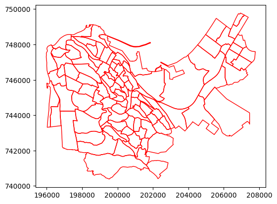
Let us plot the resulting layer to see that we are on the right track:

stat.plot(color='none', edgecolor='red');

Digital Elevation Model

Next, we will import the DEM of the Haifa area, we created earlier (see Writing rasters), creating a file connection named src:

src = rasterio.open('output/carmel.tif')

and reading the values into an array named r. Recall that r is a two-dimensional array of type int, where the value -9999 marks “No Data”:

r = src.read(1)
r

array([[-9999, -9999, -9999, ..., -9999, -9999, -9999],
       [-9999, -9999, -9999, ..., -9999, -9999, -9999],
       [-9999, -9999, -9999, ..., -9999, -9999, -9999],
       ...,
       [-9999, -9999, -9999, ..., -9999, -9999, -9999],
       [-9999, -9999, -9999, ..., -9999, -9999, -9999],
       [-9999, -9999, -9999, ..., -9999, -9999, -9999]], dtype=int16)

Transforming to same CRS

Any spatial operation that involves two spatial layers requires that they are in the same CRS. Examining the CRS reveals that the stat layer is in ITM:

stat.crs

<Derived Projected CRS: EPSG:2039>
Name: Israel 1993 / Israeli TM Grid
Axis Info [cartesian]:
- E[east]: Easting (metre)
- N[north]: Northing (metre)
Area of Use:
- name: Israel - onshore; Palestine Territory - onshore.
- bounds: (34.17, 29.45, 35.69, 33.28)
Coordinate Operation:
- name: Israeli TM
- method: Transverse Mercator
Datum: Israel 1993
- Ellipsoid: GRS 1980
- Prime Meridian: Greenwich

whereas the dem raster is in UTM:

src.crs

CRS.from_epsg(32636)

Therefore, we will transform the stat layer to the CRS of the raster (i.e., UTM), using the .to_crs method (see Reprojecting with .to_crs):

stat = stat.to_crs(src.crs)
stat

	STAT11	SHEM_YISHUV	geometry
1051	324.0	חיפה	MULTIPOLYGON (((687598.654 3632...
1052	331.0	חיפה	MULTIPOLYGON (((687164.328 3632...
1053	332.0	חיפה	MULTIPOLYGON (((686895.989 3632...
1054	333.0	חיפה	MULTIPOLYGON (((686645.312 3632...
1055	334.0	חיפה	MULTIPOLYGON (((686384.704 3633...
...	...	...	...
1906	621.0	חיפה	MULTIPOLYGON (((686805.960 3631...
1907	622.0	חיפה	MULTIPOLYGON (((687171.572 3631...
1908	623.0	חיפה	MULTIPOLYGON (((687362.646 3631...
1909	631.0	חיפה	MULTIPOLYGON (((687317.320 3631...
1910	632.0	חיפה	MULTIPOLYGON (((686735.397 3632...

105 rows × 3 columns

In principle we could also transform the raster to match the CRS of the vector layer, i.e., reproject the raster to ITM. However, raster reprojection involves resampling (to keep the raster regular), which inevitably distorts the distribution of raster values. Therefore, the general recommendation is to avoid raster reprojection as much as possible, preferring reprojection of the vector layer(s) to match the raster, and not vice versa.

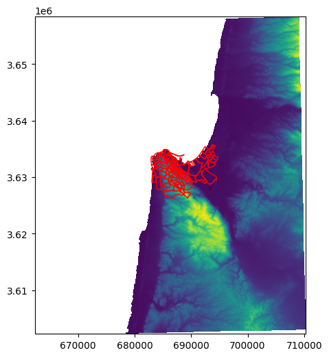
Here is a plot of both the raster and vector layer (see Plotting a raster and a vector layer), showing that they are indeed aligned:

fig, ax = plt.subplots()
rasterio.plot.show(src, ax=ax)
stat.plot(ax=ax, edgecolor='red', color='none');

Zonal statistics

Overview

In this section, we demonstrate extraction of raster values according to a polygonal layer, also known as zonal statistics. Extracting raster values according to a polygon layer involves summarizing, or aggregating, the raster values, because the polygons cover a (variable) number of raster pixels. Using a summary function, such as 'sum' or 'mean', we obtain a single “summary” value per polygonal feature.

The rasterio package is not natively integrated with geopandas, therefore to combine rasters and vector layers in the same operation we often need do one of the following:

• Process the vector layer with other methods that rasterio is compatible with (such as shapely)

• Use a third-party package that facilitates the raster-vector integration

As an example of the second approach, the operation of zonal statistics can be facilitated with the rasterstats package. The rasterstats works with rasterio rasters and geopandas vector layers. Given a raster and a vector layer, it can return a summary of pixel values, per feature, summarized withe user-specified functions.

In the example, we are going to calculate zonal statistics (mean, minimum, and maximum) of elevation (see Digital Elevation Model) per statistical area of Haifa (see Statistical areas of Haifa), which we created above. We will go through two steps:

• Calculating zonal statistics—Actually calculating the zonal statistics, using the rasterstast package

• Merging with polygon layer—Attaching the statistics back to the polygonal layer of statistical areas (stat)

Calculating zonal statistics

To calculate zonal statistics, we use the rasterstats.zonal_stats function, from the rasterstats package which we loaded earlier (see Loading raster packages). The zonal_stats function requires several inputs, as follows:

• The polygon layer that defines the areas where raster values are sampled. This can be a GeoDataFrame object, such as stat, or a GeoSeries.

• The array with raster data to be extracted. This needs to be a ndarray object, such as r.

• nodata—The array value which specifies “No Data” in the array, such as -9999.

• affine—The georeferencing matrix as defined in rasterio, such as src.transform.

• stats—a list of functions used to summarize raster values per polygon layer feature, such as ["mean","min","max"].

Other useful summary functions for the stats parameter of zonal_stats include:

• "count"—The number of valid (i.e., excluding “No Data”) pixels

• "nodata"—The number of pixels with “No Data”

• "majority"—The most frequently occurring value

• "median"—The median value

Defining custom summary functions is also possible. Keep in mind that the calculation of the statistics ignores any “No Data” values.

Here is the zonal_stats function call in our case:

result = rasterstats.zonal_stats(
    stat, 
    r, 
    nodata = src.nodata, 
    affine = src.transform, 
    stats = ['mean', 'min', 'max']
)

The returned object, result, is a list:

type(result)

list

where each element is a dict, containing the summary statistics per feature. For example, result[0] contains the minimum, maximum, and mean elevation in the first three statistical areas:

result[:3]

[{'min': 5.0, 'max': 30.0, 'mean': 13.117647058823529},
 {'min': 15.0, 'max': 52.0, 'mean': 35.72727272727273},
 {'min': 41.0, 'max': 71.0, 'mean': 53.785714285714285}]

A list of dictionaries with repeated keys can be converted to a DataFrame, where the dictionaries comprise rows. This is a data structure we are more comfortable to work with, using the methods we learned so far. The conversion is done using the pd.DataFrame function:

result = pd.DataFrame(result)
result

	min	max	mean
0	5.0	30.0	13.117647
1	15.0	52.0	35.727273
2	41.0	71.0	53.785714
3	10.0	64.0	33.300000
4	7.0	62.0	27.448980
...	...	...	...
100	128.0	248.0	182.166667
101	113.0	209.0	160.360000
102	145.0	219.0	180.708333
103	87.0	135.0	106.545455
104	66.0	102.0	82.478261

105 rows × 3 columns

Merging with polygon layer

Our last step is to combine the zonal statistics DataFrame with the original vector layer, so that we have those values side-by-side with the geometries and any other attributes we have in the vector layer. This is basically a pd.concat operation of columns in a GeoDataFrame and columns in a DataFrame. However, we need to be careful with the index. As mentioned in Concatenation by column, the indices of concatenated tables must match, since concatenation takes place by index rather than by position. Here, we have an example where indices indeed do not match, because the subsetting operation we made earlier (selecting “Haifa”, see Statistical areas of Haifa) modified the index:

result.index

RangeIndex(start=0, stop=105, step=1)

stat.index

Index([1051, 1052, 1053, 1054, 1055, 1056, 1057, 1058, 1059, 1060,
       ...
       1901, 1902, 1903, 1904, 1905, 1906, 1907, 1908, 1909, 1910],
      dtype='int64', length=105)

To make the indices match, we can “reset” (see Resetting the index) the indices of stat so that they are consecutive starting from zero, same as in result:

stat = stat.reset_index(drop=True)
stat

	STAT11	SHEM_YISHUV	geometry
0	324.0	חיפה	MULTIPOLYGON (((687598.654 3632...
1	331.0	חיפה	MULTIPOLYGON (((687164.328 3632...
2	332.0	חיפה	MULTIPOLYGON (((686895.989 3632...
3	333.0	חיפה	MULTIPOLYGON (((686645.312 3632...
4	334.0	חיפה	MULTIPOLYGON (((686384.704 3633...
...	...	...	...
100	621.0	חיפה	MULTIPOLYGON (((686805.960 3631...
101	622.0	חיפה	MULTIPOLYGON (((687171.572 3631...
102	623.0	חיפה	MULTIPOLYGON (((687362.646 3631...
103	631.0	חיפה	MULTIPOLYGON (((687317.320 3631...
104	632.0	חיפה	MULTIPOLYGON (((686735.397 3632...

105 rows × 3 columns

stat.index

RangeIndex(start=0, stop=105, step=1)

Now we can safely use pd.concat:

stat = pd.concat([stat, result], axis=1)
stat

	STAT11	SHEM_YISHUV	geometry	min	max	mean
0	324.0	חיפה	MULTIPOLYGON (((687598.654 3632...	5.0	30.0	13.117647
1	331.0	חיפה	MULTIPOLYGON (((687164.328 3632...	15.0	52.0	35.727273
2	332.0	חיפה	MULTIPOLYGON (((686895.989 3632...	41.0	71.0	53.785714
3	333.0	חיפה	MULTIPOLYGON (((686645.312 3632...	10.0	64.0	33.300000
4	334.0	חיפה	MULTIPOLYGON (((686384.704 3633...	7.0	62.0	27.448980
...	...	...	...	...	...	...
100	621.0	חיפה	MULTIPOLYGON (((686805.960 3631...	128.0	248.0	182.166667
101	622.0	חיפה	MULTIPOLYGON (((687171.572 3631...	113.0	209.0	160.360000
102	623.0	חיפה	MULTIPOLYGON (((687362.646 3631...	145.0	219.0	180.708333
103	631.0	חיפה	MULTIPOLYGON (((687317.320 3631...	87.0	135.0	106.545455
104	632.0	חיפה	MULTIPOLYGON (((686735.397 3632...	66.0	102.0	82.478261

105 rows × 6 columns

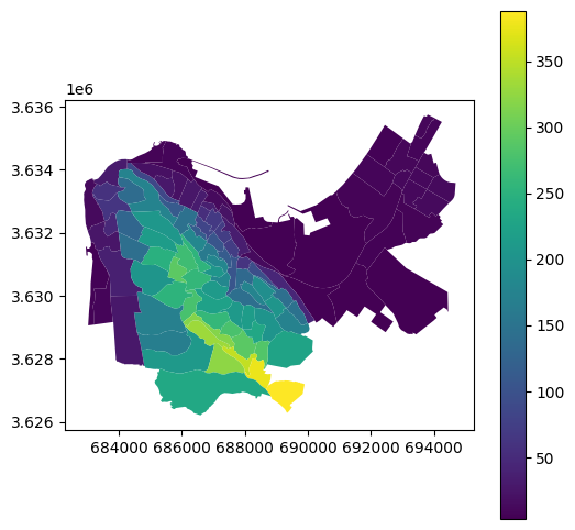
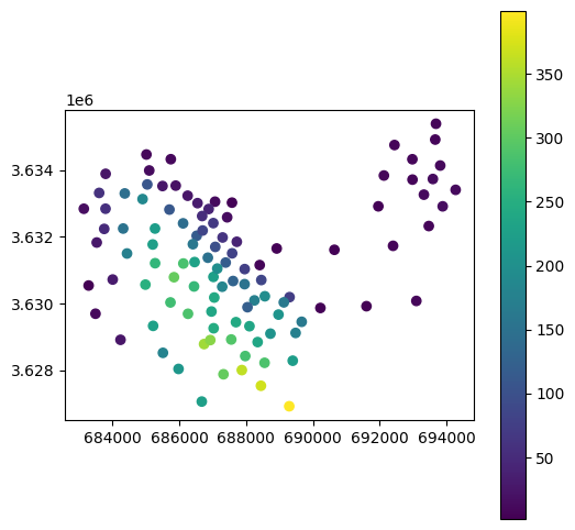
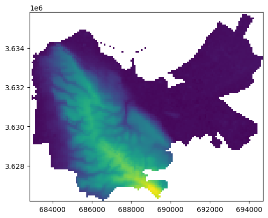
Here is a visulization of the zonal statistics result. The colors reflect the average elevation within each statistical area:

stat.plot(column='mean', legend=True);

Extracting to points

Using rasterstats

The second commonly used variant of raster data extraction is extracting values to points. Extraction to points is conceptuially simpler than extracting to polygons (see Zonal statistics), because each point corresponds to just one raster value—the value of the pixel where the point falls in. Therefore, there is no need to summarize the extracted values.

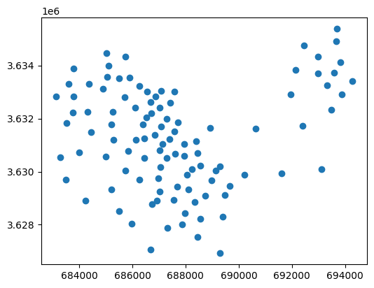
Before we begin, let us create a GeoSeries of type "Point" to demonstrate sampling of elevation values to points. For example, we can take a GeoSeries of statistical area centroids pnt:

pnt = stat.centroid
pnt

0      POINT (687071.047 3633050.615)
1      POINT (686881.442 3632830.238)
2      POINT (686685.459 3632620.552)
3      POINT (686547.304 3633006.256)
4      POINT (686252.055 3633228.654)
                    ...              
100    POINT (686408.245 3631777.877)
101    POINT (686856.572 3631373.063)
102    POINT (687138.866 3631048.022)
103    POINT (687078.293 3631697.326)
104    POINT (686700.041 3632186.932)
Length: 105, dtype: geometry

pnt.plot();

The rasterstats package has function called rasterstats.point_query, very similar in design to the rasterstats.zonal_stats function (see Calculating zonal statistics). The principal difference is that we do not need to specify summary functions (stats), since each point corresponds to a single value and there is no need to “summarize” anything. Instead, there is an additional important argument interpolate, where we specify the type of interpolation:

• 'bilinear'—Weighted average of four nearest pixels

• 'nearest'—Value of the pixel that the point falls in

Typically we prefer to use 'nearest' method, since it preserves the original raster values rather than averaging them.

For example, the following expression samples the elevation values from the Haifa DEM according to the statistical area centroids pnt:

result = rasterstats.point_query(
    pnt, 
    r, 
    nodata=src.nodata, 
    affine=src.transform,
    interpolate='nearest'
)

The result is a list of numeric elevations values:

result[:5]

[13, 42, 52, 33, 24]

We can “attach” it to the point geometries, as follows:

result = gpd.GeoDataFrame({'elev': result, 'geometry': pnt})
result

	elev	geometry
0	13	POINT (687071.047 3633050.615)
1	42	POINT (686881.442 3632830.238)
2	52	POINT (686685.459 3632620.552)
3	33	POINT (686547.304 3633006.256)
4	24	POINT (686252.055 3633228.654)
...	...	...
100	159	POINT (686408.245 3631777.877)
101	150	POINT (686856.572 3631373.063)
102	196	POINT (687138.866 3631048.022)
103	99	POINT (687078.293 3631697.326)
104	84	POINT (686700.041 3632186.932)

105 rows × 2 columns

Here is a plot of the result:

result.plot(column='elev', legend=True);

Using rasterio

Sometimes, it is preferable (or essential) to reduce the number of dependencies on third-party packages. Therefore, to expand our capabilites and our understanding of the low-level rasterio functionality, we are now going to see how the last example can be reproduced without rasterstats, relying only on geopandas and rasterio. Another benefit is flexibility: the rasterio approach supports extraction from multi-band rasters, unlike rasterstats which only supports single-band rasters.

To extract raster values to points, a rasterio raster file connection has a method called .sample. The .sample method:

• accepts a list of coordinate pairs, such as [(x,y),(x,y),...], and

• returns a list of raster value array (one per band), such as [array([band1,band2,band3]),array([band1,band2,band3]),...]

For example, suppose that we have a list with two tuples representing two points in UTM:

x = [(687071.0468361621, 3633050.615206969), (686881.4418603638, 3632830.237625203)]
x

[(687071.0468361621, 3633050.615206969),
 (686881.4418603638, 3632830.237625203)]

Using sample, we can extract the raster values at those points:

src.sample(x)

<generator object sample_gen at 0x7f1d2aa791c0>

The result is a generator object, which we can iterate over:

for i in src.sample(x):
    print(i)

[13]
[42]

or obtain all values at once into a list:

list(src.sample(x))

[array([13], dtype=int16), array([42], dtype=int16)]

Inside the list, each element is an array (of length 1, since the source raster has just one band):

list(src.sample(x))[0]

array([13], dtype=int16)

Indexing the array returns the pixel value:

list(src.sample(x))[0][0]

13

Knowing this, extracting raster values into a point GeoDataFrame is a matter of back and forth transformations, namely:

• extracting the GeoDataFrame coordinates into a list of tuples to be passed to .sample, and

• attaching the list of returned raster values back to a GeoDataFrame format

Let us begin. First, we use the .to_list method (see Conversion to list) to go from a GeoSeries to a list of shapely geometries. For example, here are the first five geometries:

pnt.to_list()[:5]

[<POINT (687071.047 3633050.615)>,
 <POINT (686881.442 3632830.238)>,
 <POINT (686685.459 3632620.552)>,
 <POINT (686547.304 3633006.256)>,
 <POINT (686252.055 3633228.654)>]

Each element in the list is a "Point" geometry. We can access its coordinates using .coords along with a conversion to list (see Point coordinates). For example, here are the coordinates of the first point:

list(pnt.to_list()[0].coords)

[(687071.0468361623, 3633050.615206969)]

Adapting the above expression into list comprehension (see List comprehension), we can extract all coordinate pairs into a plain list of tuples, as follows:

coords = [list(i.coords)[0] for i in pnt.to_list()]
coords[:5]

[(687071.0468361623, 3633050.615206969),
 (686881.441860364, 3632830.237625203),
 (686685.4586284278, 3632620.5516706416),
 (686547.3042551251, 3633006.256442973),
 (686252.0550834013, 3633228.6542930715)]

The list of coordinates (coords) can be passed to .sample. Then, we use another list comprehension to extract the values into a list called values:

values = [i[0] for i in src.sample(coords)]
values[:5]

[13, 42, 52, 33, 24]

Since we know that values is in agreement with pnt, we can safely bind them into a GeoDataFrame. We get then same result as using rasterstats.point_query (see Using rasterstats):

result = gpd.GeoDataFrame({'elev': values, 'geometry': pnt})
result

	elev	geometry
0	13	POINT (687071.047 3633050.615)
1	42	POINT (686881.442 3632830.238)
2	52	POINT (686685.459 3632620.552)
3	33	POINT (686547.304 3633006.256)
4	24	POINT (686252.055 3633228.654)
...	...	...
100	159	POINT (686408.245 3631777.877)
101	150	POINT (686856.572 3631373.063)
102	196	POINT (687138.866 3631048.022)
103	99	POINT (687078.293 3631697.326)
104	84	POINT (686700.041 3632186.932)

105 rows × 2 columns

result.plot(column='elev', legend=True);

Masking

Masking with rasterio.mask.mask

Masking a raster means “erasing” values outside an area of interest, defined using a polygon, by turning them into “No Data”. In the following example, we are going to mask the DEM raster using the layer of statistical areas of Haifa stat (see Statistical areas of Haifa).

The rasterio.mask.mask function can be used for masking. It accepts the following arguments:

• dataset—A raster file connection

• shapes—A list of shapely polygons

• crop—Whether to also reduce (i.e., crop) the raster extent according to the extent of shapes

• nodata—Value to use for “No Data”. Typically:

  • a specific value (e.g., -9999) for int rasters, or

  • np.nan for float rasters.

For example, here is how we can mask (and crop!) the DEM according to the stat polygon layer. The resulting raster has smaller extent, and the values which are outside of the statistical areas of Haifa are “erased”:

out_image, out_transform = rasterio.mask.mask(
    src, 
    stat.geometry.to_list(), 
    crop=True, 
    nodata=-9999
)

Note that rasterio.mask.mask returns a tuple, which we immediately “unpack” into two variables: out_image and out_transform.

# Tuple unpacking
a, b = (3, 12)

a

3

b

12

An alternative way to do the same, but without unpacking, could be:

result = rasterio.mask.mask(src, stat.geometry.to_list(), crop=True, nodata=-9999)
out_image = result[0]
out_transform = result[1]

Either way, the first variable, out_shape, contains the array of (cropped) raster values:

out_image

array([[[-9999, -9999, -9999, ..., -9999, -9999, -9999],
        [-9999, -9999, -9999, ..., -9999, -9999, -9999],
        [-9999, -9999, -9999, ..., -9999, -9999, -9999],
        ...,
        [-9999, -9999, -9999, ..., -9999, -9999, -9999],
        [-9999, -9999, -9999, ..., -9999, -9999, -9999],
        [-9999, -9999, -9999, ..., -9999, -9999, -9999]]], dtype=int16)

The second variable, out_transform, contains the transformation matrix:

out_transform

Affine(90.0, 0.0, 682837.0,
       0.0, -90.0, 3635822.0)

Note that out_image is a three-dimensional array (with one “layer”). For simplicity, we can transform it “back” to a two-dimensional array, by subsetting the first and only band:

out_image = out_image[0]
out_image

array([[-9999, -9999, -9999, ..., -9999, -9999, -9999],
       [-9999, -9999, -9999, ..., -9999, -9999, -9999],
       [-9999, -9999, -9999, ..., -9999, -9999, -9999],
       ...,
       [-9999, -9999, -9999, ..., -9999, -9999, -9999],
       [-9999, -9999, -9999, ..., -9999, -9999, -9999],
       [-9999, -9999, -9999, ..., -9999, -9999, -9999]], dtype=int16)

Exercise 11-c

• Why do you think we a new transformation matrix is returned? (Can we use the original transformation matrix instead?)

Here is a visualization of the result:

rasterio.plot.show(out_image, transform=out_transform);

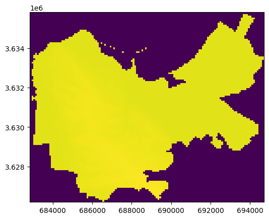
The extreme value of “No Data” (-9999) obscures the variataion of valid pixels. One way to address this is to switch to float representation, where “No Data” values can be replaced with np.nan (see exercise below). Another way to address this is to write the raster to file, where the value of “No Data” is documented, and then reproduce the plot use a file connection (see Exporting masked raster).

Exercise 11-c

• Convert the above image to float, replace "No Data" values with np.nan, and plot the result (Fig. 67).

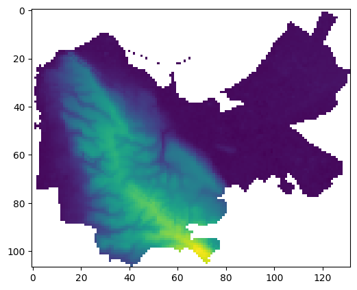
Fig. 67 Solution of exercise-11-c: Masked array of carmel.tif after conversion to float and replacing “No Data” with np.nan

Exercise 11-d

• Repeat the last exercise, but this time use crop=False inside rasterio.mask.mask (Fig. 68).

• Explain the difference between the two options, crop=True and crop=False.

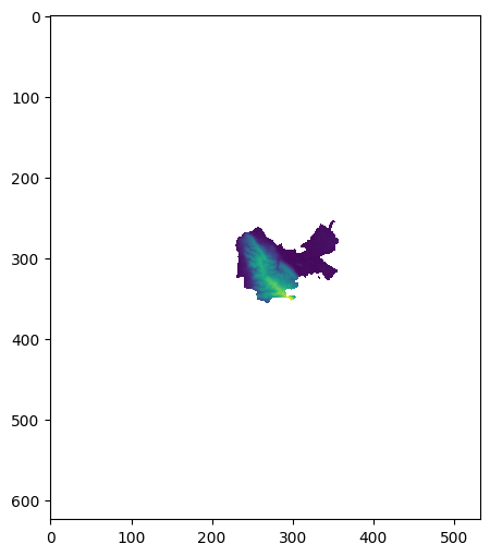
Fig. 68 Solution of exercise-11-d: Same as the last figure, but using crop=False

Exporting masked raster

To export the masked and cropped raster to file, we first need to update the metadata object according to the properties which have changed (see Writing rasters). In this case, through masking and cropping we changed the raster dimensions (height, width) and the transformation matrix (transform). Therefore:

meta = src.meta
meta.update(height=out_image.shape[0])
meta.update(width=out_image.shape[1])
meta.update(transform=out_transform)
meta

{'driver': 'GTiff',
 'dtype': 'int16',
 'nodata': -9999.0,
 'width': 132,
 'height': 107,
 'count': 1,
 'crs': CRS.from_epsg(32636),
 'transform': Affine(90.0, 0.0, 682837.0,
        0.0, -90.0, 3635822.0)}

Now we can write the out_image to file, which we name carmel_cropped.tif:

new_dataset = rasterio.open('output/carmel_cropped.tif', 'w', **meta)
new_dataset.write(out_image, 1)
new_dataset.close()

Let us try to read back the result and plot it, which has the advantage of showing “No Data” values in white color:

src_carmel_cropped = rasterio.open('output/carmel_cropped.tif')
rasterio.plot.show(src_carmel_cropped);

Note

For more details about masking with rasterio, see the dicumentation: https://rasterio.readthedocs.io/en/latest/topics/masking-by-shapefile.html

Raster to polygons

Overview

The last raster-vector operation we are going to explore in this chapter is the conversion from raster to a vector layer. In general, there are three types of conversions:

• Raster to points

• Raster to polygons

• Raster to contours

The first two conversions are straightforward. Essentially, each raster pixel is transformed to a point, or to a polygon, resulting in a point or polygon layer, respectively. Additionally, in a raster to polygons conversion, adjacent pixels with identical values are typically dissolved into larger polygons. The raster to contours conversion is different, as the resulting layer does not represent pixel geometry directly, but through a contour algorithm, which is beyond the scope of rasterio.

In this section, we demonstrate the raster to polygons conversion. We leave the raster to points conversion as an exercise for the reader (Fig. 70). The raster to contours conversion is beyond the scope of this book.

The rasterio.features.shapes function

The rasterio.features.shapes function gives access to the raster pixel geometries, as polygons, and their values. The returned object is an iterator (more specifically, a generator), which yields geometry,value pairs. We can use mask to filter the geometries. Furthermore, we must use transform to yield true spatial coordinates of the polygons.

For example, the following expression returns a generator named shapes, referring to all pixels with values greater than 525 in the r array (i.e., pixels with elevation above 525 \(m\)):

shapes = rasterio.features.shapes(r, mask=r>525, transform=src.transform)
shapes

<generator object shapes at 0x7f1d2a69b680>

We can generate all shapes at once, into a list named pol, as follows:

pol = list(shapes)

Each element in pol is a tuple of length 2, containing:

• The GeoJSON-like dict representing the polygon geometry

• The value of the pixel(s) which comprise the polygon

For example:

pol[0]

({'type': 'Polygon',
  'coordinates': [[(690397.0, 3625022.0),
    (690397.0, 3624932.0),
    (690487.0, 3624932.0),
    (690487.0, 3625022.0),
    (690397.0, 3625022.0)]]},
 526.0)

The GeoJSON-like dict:

pol[0][0]

{'type': 'Polygon',
 'coordinates': [[(690397.0, 3625022.0),
   (690397.0, 3624932.0),
   (690487.0, 3624932.0),
   (690487.0, 3625022.0),
   (690397.0, 3625022.0)]]}

can be directly translated to a shapely geometry using shapely.geometry.shape (shapely from GeoJSON-like dict):

x = shapely.geometry.shape(pol[0][0])
x

The second element in the tuple, the pixel value, is a plain number:

pol[0][1]

526.0

Raster to GeoDataFrame

Going from a list of geometries and associated values to a GeoDataFrame is something we already know how to do (see List comprehension, Creating a GeoSeries, Creating a DataFrame, and Creating a GeoDataFrame). First, we extract just the geometries into a list, and transform it to a GeoSeries:

geom = [shapely.geometry.shape(i[0]) for i in pol]
geom = gpd.GeoSeries(geom, crs=src.crs)
geom

0     POLYGON ((690397.000 3625022.00...
1     POLYGON ((690487.000 3625022.00...
2     POLYGON ((690577.000 3624932.00...
3     POLYGON ((692017.000 3623852.00...
4     POLYGON ((692017.000 3623762.00...
                     ...                
40    POLYGON ((693007.000 3622502.00...
41    POLYGON ((693727.000 3622052.00...
42    POLYGON ((693817.000 3622052.00...
43    POLYGON ((693817.000 3621962.00...
44    POLYGON ((693907.000 3621962.00...
Length: 45, dtype: geometry

Then, we extract just the values into a list, and transform it to a Series:

values = [i[1] for i in pol]
values = pd.Series(values)
values

0     526.0
1     527.0
2     526.0
3     527.0
4     528.0
      ...  
40    527.0
41    529.0
42    527.0
43    528.0
44    529.0
Length: 45, dtype: float64

Finally, we combine the two—the Series and the GeoSeries—into a GeoDataFrame:

result = gpd.GeoDataFrame({'elev': values, 'geometry': geom})
result

	elev	geometry
0	526.0	POLYGON ((690397.000 3625022.00...
1	527.0	POLYGON ((690487.000 3625022.00...
2	526.0	POLYGON ((690577.000 3624932.00...
3	527.0	POLYGON ((692017.000 3623852.00...
4	528.0	POLYGON ((692017.000 3623762.00...
...	...	...
40	527.0	POLYGON ((693007.000 3622502.00...
41	529.0	POLYGON ((693727.000 3622052.00...
42	527.0	POLYGON ((693817.000 3622052.00...
43	528.0	POLYGON ((693817.000 3621962.00...
44	529.0	POLYGON ((693907.000 3621962.00...

45 rows × 2 columns

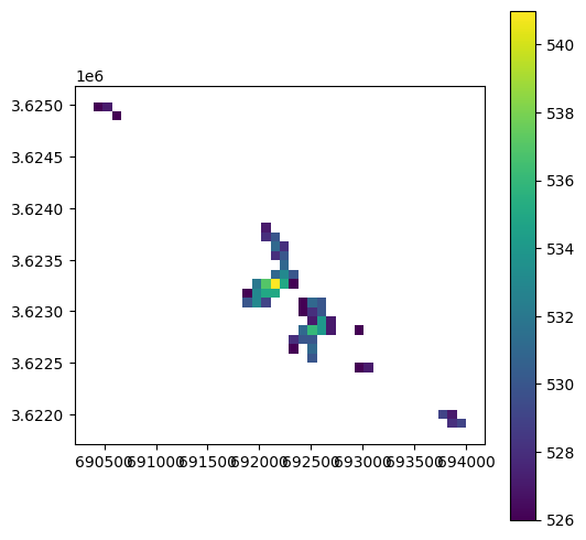
Here is a plot of the result, the DEM pixels that are above 525 \(m\) as polygons:

result.plot(column='elev', legend=True);

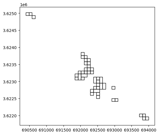
Plotting just the geometries, without symbology, reveals the dissoving of neighboring pixels where elevation is identical:

result.plot(color='none');

Exercise 11-e

• Dissolve the above polygon layer into a single 'MultiPolygon' geometry and plot it (Fig. 69).

• What is the total area with alevation above 525 \(m\)? (answer: 421200.0)

• How many separate 'Polygon' geometries is the dissolved 'MultiPolygon' composed of? (answer: 7)

Fig. 69 Solution of exercise-11-e: “Raster to polygons” result dissoved

Exercise 11-f

• Create a point layer of the pixels with elevation above 525 \(m\). The result should be a GeoDataFrame of type 'Point', with an attribute named 'elev' reflecting the elevation of each point.

• Plot the result, with symbology according to 'elev' (Fig. 70)

• Hint: you can replace the r array values with sequential values (so that no pixels are dissolved), transform to polygons, then calculate the polygon centroids, and finally extract elevation values to those points.

Fig. 70 Solution of exercise-11-f: “Raster to points” result

Note

The opposite transformation, i.e., from vector layer to raster, is known as rasterizing. Technically, rasterizing implies “burning” vector layer attribute values into a template raster, at those pixels covered by the vector layer. See the Burning shapes into a raster entry in the rasterio documentation for details.

More exercises

Exercise 11-g

• Calculate the proportion of land area that is above elevation of 100 \(m\), for each statistical area of Haifa, according to the same polygon layer and DEM as in Zonal statistics.

• To do that, first classify the DEM to values to 0 (below 100 \(m\) or “No Data”) and 1 (above 100 \(m\)). Then, calculate the zonal average of the zeroes and ones per statistical area. The resulting values are going to be equal to the proportion of pixels (i.e., proportion of area) that is above 100 \(m\).

• Show the results on a map (Fig. 71).

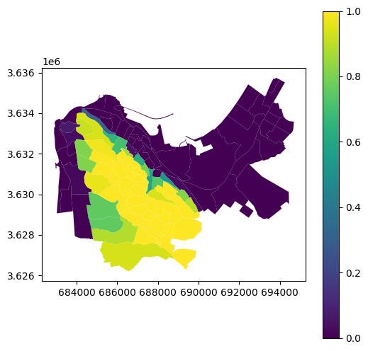
Fig. 71 Solution of exercise-11-g: Proportion of land area above 400 m in statistical areas of Haifa

Exercise 11-h

• Calculate and plot the average spectral profile (in blue, green, red, and NIR) of "Be'er Sheva", "Lehavim", "Omer", "Lakiye", and "Segev Shalom", according to the towns layer (muni_il.shp, names in the "Muni_Eng" column) and the multi-spectral Sentinel-2 image (sentinel2.tif) (Fig. 72).

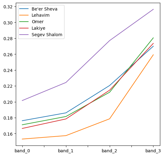
Fig. 72 Solution of exercise-11-h: Spectral profiles of four towns

Exercise solutions

Exercise 11-c

import numpy as np
import geopandas as gpd
import rasterio
import rasterio.mask
import rasterio.plot
# Prepare raster
src = rasterio.open('output/carmel.tif')
# Prepare polygons
stat = gpd.read_file('data/statisticalareas_demography2019.gdb')
stat = stat[['STAT11', 'SHEM_YISHUV', 'geometry']]
sel = stat['SHEM_YISHUV'] == 'חיפה'
stat = stat[sel]
stat = stat.to_crs(src.crs)
# Mask
out_image, out_transform = rasterio.mask.mask(src, stat.geometry.to_list(), crop=True, nodata=-9999)
out_image = out_image[0]
# To 'float'
out_image1 = out_image.astype(float)
out_image1[out_image1 == -9999] = np.nan
# Plot
rasterio.plot.show(out_image1);

Exercise 11-e

import pandas as pd
import shapely
import geopandas as gpd
import rasterio
import rasterio.mask
from rasterio.plot import show
# Prepare raster
src = rasterio.open('output/carmel.tif')
r = src.read(1)
# Prepare polygons
stat = gpd.read_file('data/statisticalareas_demography2019.gdb')
stat = stat[['STAT11', 'SHEM_YISHUV', 'geometry']]
sel = stat['SHEM_YISHUV'] == 'חיפה'
stat = stat[sel]
stat = stat.to_crs(src.crs)
# Raster to polygons
shapes = rasterio.features.shapes(r, mask=r > 525, transform=src.transform)
pol = list(shapes)
geom = [shapely.geometry.shape(i[0]) for i in pol]
geom = gpd.GeoSeries(geom, crs=src.crs)
values = [i[1] for i in pol]
values = pd.DataFrame({'elev': values})
result = gpd.GeoDataFrame(data=values, geometry=geom)
# Dissolve
result = result.unary_union
result

result.area

Exercise 11-d

import numpy as np
import geopandas as gpd
import rasterio
import rasterio.mask
import rasterio.plot
# Prepare raster
src = rasterio.open('output/carmel.tif')
# Prepare polygons
stat = gpd.read_file('data/statisticalareas_demography2019.gdb')
stat = stat[['STAT11', 'SHEM_YISHUV', 'geometry']]
sel = stat['SHEM_YISHUV'] == 'חיפה'
stat = stat[sel]
stat = stat.to_crs(src.crs)
# Mask
out_image, out_transform = rasterio.mask.mask(src, stat.geometry.to_list(), crop=False, nodata=-9999)
out_image = out_image[0]
# To 'float'
out_image1 = out_image.astype(float)
out_image1[out_image1 == -9999] = np.nan
# Plot
rasterio.plot.show(out_image1);

Exercise 11-f

import numpy as np
import rasterio
import shapely
import rasterstats
import geopandas as gpd
# Prepare raster
src = rasterio.open('output/carmel.tif')
r = src.read(1)
r1 = r.copy()
r1[r > 525] = np.arange(0, r[r > 525].size)
# Raster to polygons
shapes = rasterio.features.shapes(r1, mask=r > 525, transform=src.transform)
pol = list(shapes)
geom = [shapely.geometry.shape(i[0]) for i in pol]
geom = gpd.GeoSeries(geom, crs=src.crs)
# Polygons to points
geom = geom.centroid
result = gpd.GeoDataFrame(geometry=geom)
# Extract values to points
x = rasterstats.point_query(
    result, 
    r, 
    nodata = src.nodata, 
    affine = src.transform,
    interpolate='nearest'
)
result['elev'] = x
# Plot
result.plot(column='elev', legend=True);

Exercise 11-g

import pandas as pd
import geopandas as gpd
import rasterio
from rasterstats import zonal_stats
# Prepare raster
src = rasterio.open('output/carmel.tif')
r = src.read(1)
r[(r != -9999) & (r < 100)] = 0
r[r >= 100] = 1
# Prepare polygons
stat = gpd.read_file('data/statisticalareas_demography2019.gdb')
stat = stat[['SHEM_YISHUV', 'STAT11', 'geometry']]
sel = stat['SHEM_YISHUV'] == 'חיפה'
stat = stat[sel]
stat = stat.reset_index(drop = True)
stat = stat.to_crs(src.crs)
# Extract
result = zonal_stats(stat, r, nodata=-9999, affine=src.transform, stats='mean')
result = pd.DataFrame(result)
stat1 = pd.concat([stat, result], axis=1)
# Plot
stat1.plot(column="mean", legend=True);

Exercise 11-h

import pandas as pd
import geopandas as gpd
import rasterio
from rasterstats import zonal_stats
# Prepare raster
src = rasterio.open('output/sentinel2.tif')
r = src.read()
r = r / 10000
# Prepare polygons
pol = gpd.read_file('data/muni_il.shp')
pol = pol[['Muni_Eng', 'geometry']]
sel = ["Be'er Sheva", "Lehavim", "Omer", "Lakiye", "Segev Shalom"]
pol = pol[pol["Muni_Eng"].isin(sel)]
pol = pol.to_crs(src.crs)
# Extract
result = []
for band in range(r.shape[0]):
    tmp = zonal_stats(pol, r[band], nodata=-9999, affine=src.transform, stats='mean')
    tmp = pd.DataFrame(tmp)
    tmp = tmp.rename(columns = {'mean': 'band_' + str(band)})
    tmp.index = sel
    result.append(tmp)
result = pd.concat(result, axis=1)
# Plot
result.T.plot();