Table reshaping and joins

Last updated: 2024-12-09 14:55:04

---

Introduction

In the previous chapter (see Tables (pandas)), we introduced the pandas package, and covered the basic operations with tables using pandas, such as importing and exporting, subsetting, renaming columns, sorting, and calculating new columns. In practice, we often need to do more than that. For example, we may need to aggregate, or to reshape, tables into a different form, or to combine numerous tables into one. In this chapter, we cover some of the common table operations which involve modifying table structure or combining multiple tables.

When working with data, it is often necessary to combine data from multiple sources, and/or reshape data into the right form that a particular function accepts:

• Combining may simply involve “pasting”, or concatenating, two tables one on top of the other, or side-by-side (see Concatenation).

• In more complex cases, combining involves a table join, where the information from two tables is combined according to one or more “key” columns which are common to both tables (see Joining tables).

• Moreover, we may need to summarize the values of a table according to a particular grouping, which is known as aggregation (see Aggregation).

• A special type of aggregation is applying a function across each row, or each column, of a table (Row/col-wise operations).

In this chapter, we learn about all of those common methods for combining and reshaping tables. By the end of the chapter, you will have the ability to not just import and transform tables in Python (see Tables (pandas)), but also to reshape and combine tables to the right form, which facilitates further analysis and insight from the data in those tables.

Sample data

First, let’s recreate the small table named stations which we used in the previous chapter (see Creating a DataFrame):

import numpy as np
import pandas as pd
name = pd.Series(['Beer-Sheva Center', 'Beer-Sheva University', 'Dimona'])
city = pd.Series(['Beer-Sheva', 'Beer-Sheva', 'Dimona'])
lines = pd.Series([4, 5, 1])
piano = pd.Series([False, True, False])
lon = pd.Series([34.798443, 34.812831, 35.011635])
lat = pd.Series([31.243288, 31.260284, 31.068616])
d = {'name': name, 'city': city, 'lines': lines, 'piano': piano, 'lon': lon, 'lat': lat}
stations = pd.DataFrame(d)
stations

	name	city	lines	piano	lon	lat
0	Beer-Sheva Center	Beer-Sheva	4	False	34.798443	31.243288
1	Beer-Sheva University	Beer-Sheva	5	True	34.812831	31.260284
2	Dimona	Dimona	1	False	35.011635	31.068616

We will also load the sample climatic data which we are also familiar with from the previous chapter (Reading from file), into a DataFrame named dat:

dat = pd.read_csv('data/ZonAnn.Ts+dSST.csv')
dat

	Year	Glob	NHem	SHem	24N-90N	...	EQU-24N	24S-EQU	44S-24S	64S-44S	90S-64S
0	1880	-0.17	-0.28	-0.05	-0.38	...	-0.14	-0.11	-0.04	0.05	0.67
1	1881	-0.09	-0.18	0.00	-0.36	...	0.11	0.10	-0.06	-0.07	0.60
2	1882	-0.11	-0.21	-0.01	-0.31	...	-0.04	-0.05	0.01	0.04	0.63
3	1883	-0.17	-0.28	-0.07	-0.34	...	-0.17	-0.16	-0.04	0.07	0.50
4	1884	-0.28	-0.42	-0.15	-0.61	...	-0.12	-0.17	-0.19	-0.02	0.65
...	...	...	...	...	...	...	...	...	...	...	...
139	2019	0.98	1.20	0.75	1.42	...	0.90	0.90	0.75	0.39	0.83
140	2020	1.01	1.35	0.68	1.67	...	0.88	0.84	0.58	0.39	0.89
141	2021	0.85	1.14	0.56	1.42	...	0.72	0.60	0.72	0.32	0.30
142	2022	0.89	1.16	0.62	1.52	...	0.62	0.51	0.79	0.38	1.09
143	2023	1.17	1.49	0.85	1.78	...	1.07	1.04	0.91	0.44	0.63

144 rows × 15 columns

Concatenation

Overview

The most basic method for combining several tables into one is concatenation, which essentially means binding tables one on top of another, or side-by-side:

• Concatenation by row is usually desired when the two (or more) tables share exactly the same columns. For example, combining several tables reflecting the same data (e.g., measured on different dates, or for different subjects) involves concatenation by row.

• Concatenation by column is useful when we need to attach new variables for the same observations we already have. For example, we may want to combine several different types of observations which are split across separate files.

In pandas, concatenation can be done using pd.concat. The pd.concat function accepts a list of tables, which are combined:

• By row when using axis=0 (the default)

• By column when using axis=1

Concatenation by row

To demonstrate concatenation by row, let’s create two subsets x and y of stations, with the 1^st row and the 2^nd-3^rd rows, respectively:

x = stations.iloc[[0], :]     ## 1st row
x

	name	city	lines	piano	lon	lat
0	Beer-Sheva Center	Beer-Sheva	4	False	34.798443	31.243288

y = stations.iloc[[1, 2], :]  ## 2nd and 3rd rows
y

	name	city	lines	piano	lon	lat
1	Beer-Sheva University	Beer-Sheva	5	True	34.812831	31.260284
2	Dimona	Dimona	1	False	35.011635	31.068616

The expression pd.concat([x,y]) can then be used to concatenate x and y, by row, re-creating the complete table stations:

pd.concat([x, y])

	name	city	lines	piano	lon	lat
0	Beer-Sheva Center	Beer-Sheva	4	False	34.798443	31.243288
1	Beer-Sheva University	Beer-Sheva	5	True	34.812831	31.260284
2	Dimona	Dimona	1	False	35.011635	31.068616

Note that pd.concat accepts a list of DataFrames to concatenate, such as [x,y]. In this example the list is of length 2, but in general it can be of any length.

Concatenation by column

To demonstrate concatenation by column, let’s now split stations to subsets x and y by column. For example, the x table is going to contain one column 'name':

x = stations[['name']]
x

	name
0	Beer-Sheva Center
1	Beer-Sheva University
2	Dimona

and the y table is going to contain two columns 'lon' and 'lat':

y = stations[['lon', 'lat']]
y

	lon	lat
0	34.798443	31.243288
1	34.812831	31.260284
2	35.011635	31.068616

To concatenate by column, we use pd.concat with the axis=1 argument. This concatenates the tables x and y side-by-side:

pd.concat([x, y], axis=1)

	name	lon	lat
0	Beer-Sheva Center	34.798443	31.243288
1	Beer-Sheva University	34.812831	31.260284
2	Dimona	35.011635	31.068616

Alignment by index

Note that concatenation—like many other operations in pandas—operates based on the index, rather than position. This is not a problem when concatenating by row, where columns typically need to be aligned by their index, i.e., column name (see Concatenation by row). When concatenating by column, however, we need to pay attention to the index: is it meaningful, and we want to use it when aligning rows? Or is it arbitarary, and we want to reset it before concatenating?

For example, here is what happens in concatenation by column, when the index is not aligned (see Setting Series index):

y.index = [1,2,3]
pd.concat([x, y], axis=1)

	name	lon	lat
0	Beer-Sheva Center	NaN	NaN
1	Beer-Sheva University	34.798443	31.243288
2	Dimona	34.812831	31.260284
3	NaN	35.011635	31.068616

To make sure we concatenate based on position, we may reset the index (using .reset_index(drop=True)) on both tables before concatenation:

y = y.reset_index(drop=True)
pd.concat([x, y], axis=1)

	name	lon	lat
0	Beer-Sheva Center	34.798443	31.243288
1	Beer-Sheva University	34.812831	31.260284
2	Dimona	35.011635	31.068616

Row/col-wise operations

Built-in methods

pandas defines summary methods which can be used to calculate row-wise and column-wise summaries of DataFrames. The pandas methods are generally similar to the numpy 2D summary functions and methods (see Summaries per dimension (2D)) which we learned about earlier, but there are several important differences to keep in mind:

• pandas only has methods, not functions, i.e., there is a .mean method but there is no pd.mean function—unlike numpy, which in many cases has both, e.g., both .mean and np.mean (see Table 13)

• The default axis is different: in pandas the default is column-wise summary (axis=0), while in numpy the default is “global” summary (axis=None) (see Global summaries)

• pandas methods exclude “No Data” by default (see Operators with missing values), unless we explicitly specify skipna=False—unlike numpy which by default includes “No Data”, unless using the specific “No Data”-safe functions such as np.nanmean (see Operations with “No Data”)

Commonly used pandas summary methods are listed in Table 14.

Table 14 Pandas aggregation methods

Operation	Method
.sum	Sum
.min	Minimum
.max	Maximum
.mean	Mean
.median	Median
.count	Count (of non-missing values)
.nunique	Number of unique values
.idxmin	Index of (first) minimum
.idxmax	Index of (first) maximum
.any	Is at least one element True?
.all	Are all elements True?

For the next few examples, let’s take the regional temperature anomaly time series into a separate DataFrame named regions:

cols = [
    '90S-64S', 
    '64S-44S', 
    '44S-24S', 
    '24S-EQU', 
    'EQU-24N', 
    '24N-44N', 
    '44N-64N', 
    '64N-90N'
]
regions = dat[cols]
regions

	90S-64S	64S-44S	44S-24S	24S-EQU	EQU-24N	24N-44N	44N-64N	64N-90N
0	0.67	0.05	-0.04	-0.11	-0.14	-0.26	-0.52	-0.80
1	0.60	-0.07	-0.06	0.10	0.11	-0.19	-0.50	-0.93
2	0.63	0.04	0.01	-0.05	-0.04	-0.13	-0.31	-1.41
3	0.50	0.07	-0.04	-0.16	-0.17	-0.24	-0.58	-0.18
4	0.65	-0.02	-0.19	-0.17	-0.12	-0.45	-0.66	-1.30
...	...	...	...	...	...	...	...	...
139	0.83	0.39	0.75	0.90	0.90	0.99	1.43	2.71
140	0.89	0.39	0.58	0.84	0.88	1.19	1.81	2.88
141	0.30	0.32	0.72	0.60	0.72	1.26	1.35	2.05
142	1.09	0.38	0.79	0.51	0.62	1.27	1.50	2.34
143	0.63	0.44	0.91	1.04	1.07	1.47	1.87	2.58

144 rows × 8 columns

Using the .mean method combined with axis=0 (i.e., the function is applied on each column), we can calculate the mean temperature anomaly in each region:

regions.mean(axis=0)

90S-64S   -0.074028
64S-44S   -0.053681
44S-24S    0.047917
24S-EQU    0.083056
EQU-24N    0.066181
24N-44N    0.052500
44N-64N    0.142500
64N-90N    0.273333
dtype: float64

Note that axis=0 is the default, so we can also get the same result without specifying it (unlike numpy where the default is global summary, i.e., axis=None; see Global summaries):

regions.mean()

90S-64S   -0.074028
64S-44S   -0.053681
44S-24S    0.047917
24S-EQU    0.083056
EQU-24N    0.066181
24N-44N    0.052500
44N-64N    0.142500
64N-90N    0.273333
dtype: float64

Exercise 06-a

• Calculate a list of (the first) years when the maximum temperature was observed per region (answer: [1996, 1985, 2023, 2016, 2023, 2023, 2023, 2016])

Conversely, using axis=1, we can calculate row means, i.e., the average temperature anomaly for each year across all regions:

regions.mean(axis=1)

0     -0.14375
1     -0.11750
2     -0.15750
3     -0.10000
4     -0.28250
        ...   
139    1.11250
140    1.18250
141    0.91500
142    1.06250
143    1.25125
Length: 144, dtype: float64

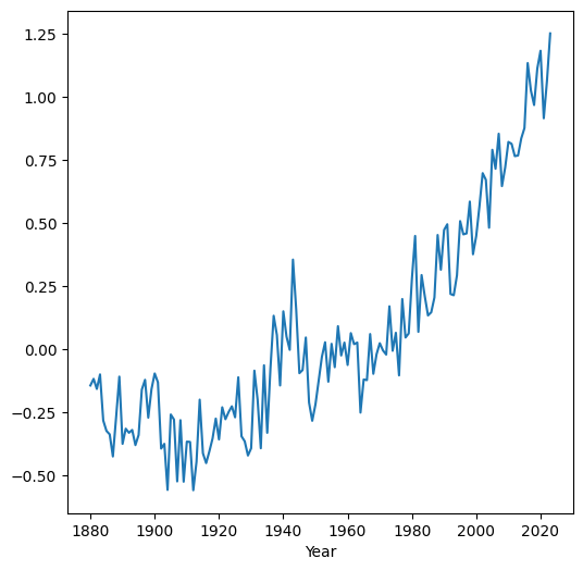
If necessary, the result can be assigned into a new column (see Creating new columns), hereby named mean, as follows:

dat['mean'] = regions.mean(axis=1)
dat

	Year	Glob	NHem	SHem	24N-90N	...	24S-EQU	44S-24S	64S-44S	90S-64S	mean
0	1880	-0.17	-0.28	-0.05	-0.38	...	-0.11	-0.04	0.05	0.67	-0.14375
1	1881	-0.09	-0.18	0.00	-0.36	...	0.10	-0.06	-0.07	0.60	-0.11750
2	1882	-0.11	-0.21	-0.01	-0.31	...	-0.05	0.01	0.04	0.63	-0.15750
3	1883	-0.17	-0.28	-0.07	-0.34	...	-0.16	-0.04	0.07	0.50	-0.10000
4	1884	-0.28	-0.42	-0.15	-0.61	...	-0.17	-0.19	-0.02	0.65	-0.28250
...	...	...	...	...	...	...	...	...	...	...	...
139	2019	0.98	1.20	0.75	1.42	...	0.90	0.75	0.39	0.83	1.11250
140	2020	1.01	1.35	0.68	1.67	...	0.84	0.58	0.39	0.89	1.18250
141	2021	0.85	1.14	0.56	1.42	...	0.60	0.72	0.32	0.30	0.91500
142	2022	0.89	1.16	0.62	1.52	...	0.51	0.79	0.38	1.09	1.06250
143	2023	1.17	1.49	0.85	1.78	...	1.04	0.91	0.44	0.63	1.25125

144 rows × 16 columns

Here is a visualization (see Line plots (pandas)) of the mean time series we just calculated:

dat.set_index('Year')['mean'].plot();

apply and custom functions

In case we need to apply a custom function on each row, or column, we can use the .apply method combined with a lambda function (see Lambda functions). For example, here is an alternative way to calculate row-wise means, using the .apply method and a lambda function. The result is the same as regions.mean() (see Built-in methods):

regions.apply(lambda x: x.mean())

90S-64S   -0.074028
64S-44S   -0.053681
44S-24S    0.047917
24S-EQU    0.083056
EQU-24N    0.066181
24N-44N    0.052500
44N-64N    0.142500
64N-90N    0.273333
dtype: float64

The advantage is that we can use any custom function definition. For example, the following expression calculates whether each region had temperature anomaly above 1 degree, in at least one of the 140 years:

regions.apply(lambda x: (x > 1).any())

90S-64S     True
64S-44S    False
44S-24S    False
24S-EQU     True
EQU-24N     True
24N-44N     True
44N-64N     True
64N-90N     True
dtype: bool

Similarly to the built-in summary functions (see Built-in methods), .apply uses the axis argument, with axis=0 specifying column-wise summaries as shown in the last two examples (the default), or axis=1 for row-wise summaries.

Exercise 06-b

• Function np.polyfit can be used to calculate the slope of linear regression between two columns. For example, using the code section shown below, you can find out that the linear trend of temperature in the '44S-24S' region was an increasing one, at 0.0066 degrees per year.

• Adapt the code into to the form of a function named slope which, given two Series objects x and y, calculates the linear slope. For example, f(dat['Year'],regions['44S-24S']) should return 0.0066.

• Use the slope function you defined within the .apply method, to calculate the slope in all columns of regions at once.

• Hint: you need to keep the x argument of slope fixed at dat['Year'], while the various columns of regions are passed to y. To do that, write another function (or use a lambda function) that “wraps” slope and runs it with just the y parameter (keeping x fixed).

x = dat['Year']
y = regions['44S-24S']
np.polyfit(x, y, 1)[0]

Joining tables

Overview

One of the most common operations when working with data is a table join. In a table join, two tables are combined into one, based on one or more common column(s). For example, when compiling a dataset about different cities, we may collect data on different aspects of each city (population size, socio-economic status, built area, etc.) from different sources. To work with these data together, the various tables need to be joined into one. The common column, in this case, would be the city name, or city ID.

When working with pandas, tables can be joined, based on one or more common column, using the pd.merge function. pd.merge has the following important parameters:

• left—The first (“left”) table

• right—The second (“right”) table

• how—The type of join, one of: 'left', 'right', 'outer', 'inner' (the default), 'cross'

• on—The name(s) of the common column(s) where identical values are considered a “match”

The type of join (the how parameter) basically determines what should be done with non-matching records. The options are 'left', 'right', 'outer', 'inner' (the default), and 'cross'. The meaning of the join types is the same as in SQL[1], and will be demonstrated through examples below.

Stations example

For a first small example, let’s get back to the stations table:

stations

	name	city	lines	piano	lon	lat
0	Beer-Sheva Center	Beer-Sheva	4	False	34.798443	31.243288
1	Beer-Sheva University	Beer-Sheva	5	True	34.812831	31.260284
2	Dimona	Dimona	1	False	35.011635	31.068616

Suppose we have another small table named status which describes the status ('Closed' or 'Open') of select stations:

name = pd.Series(['Beer-Sheva Center', 'Beer-Sheva University', 'Tel-Aviv University'])
status = pd.Series(['Closed', 'Open', 'Open'])
status = pd.DataFrame({'name': name, 'status': status})
status

	name	status
0	Beer-Sheva Center	Closed
1	Beer-Sheva University	Open
2	Tel-Aviv University	Open

The stations and status can be joined as follows:

pd.merge(stations, status)

	name	city	lines	piano	lon	lat	status
0	Beer-Sheva Center	Beer-Sheva	4	False	34.798443	31.243288	Closed
1	Beer-Sheva University	Beer-Sheva	5	True	34.812831	31.260284	Open

This implies the default, on being equal to the column(s) sharing the same name in both tables (on='name', in this case), and an 'inner' join (i.e., how='inner'). As you can see, an inner join returns just the matching rows. It is better to be explicit, for clarity:

pd.merge(stations, status, on='name', how='inner')

	name	city	lines	piano	lon	lat	status
0	Beer-Sheva Center	Beer-Sheva	4	False	34.798443	31.243288	Closed
1	Beer-Sheva University	Beer-Sheva	5	True	34.812831	31.260284	Open

Unlike an 'inner' join, a 'left' join returns all records from the first (“left”) table, even those that have no match in the second (“right”) table. For example, 'Dimona' station does not appear in the status table, but it is still returned in the result (with status set to np.nan):

pd.merge(stations, status, on='name', how='left')

	name	city	lines	piano	lon	lat	status
0	Beer-Sheva Center	Beer-Sheva	4	False	34.798443	31.243288	Closed
1	Beer-Sheva University	Beer-Sheva	5	True	34.812831	31.260284	Open
2	Dimona	Dimona	1	False	35.011635	31.068616	NaN

A 'right' join is the opposite of a 'left' join, i.e., it returns all records from the “right” table, even those that have no match in the “left” table. This time, values absent in the “left” table are set to np.nan:

pd.merge(stations, status, on='name', how='right')

	name	city	lines	piano	lon	lat	status
0	Beer-Sheva Center	Beer-Sheva	4.0	False	34.798443	31.243288	Closed
1	Beer-Sheva University	Beer-Sheva	5.0	True	34.812831	31.260284	Open
2	Tel-Aviv University	NaN	NaN	NaN	NaN	NaN	Open

Finally, an 'outer' (also known as “full”) join returns all record from both tables, regardless of whether they have a matching record in the other table. Values that have no match in both the “left” and “right” tables are set to np.nan:

pd.merge(stations, status, on='name', how='outer')

	name	city	lines	piano	lon	lat	status
0	Beer-Sheva Center	Beer-Sheva	4.0	False	34.798443	31.243288	Closed
1	Beer-Sheva University	Beer-Sheva	5.0	True	34.812831	31.260284	Open
2	Dimona	Dimona	1.0	False	35.011635	31.068616	NaN
3	Tel-Aviv University	NaN	NaN	NaN	NaN	NaN	Open

When working with data, we often have one main, or “template”, table we are working with (“left”) and we are interested to join data coming from another external (“right”) table to it. In this scenario we usually prefer not to lose any records from the “left” table. Even if some of the records have no match and get “No Data” values (namely, np.nan), we usually prefer to keep those records and deal with the missing values as necessary, rather than lose the records altogether. Therefore, a 'left' join is often most useful in data analysis. For example, in the above situation a 'left' join makes sense if our focus is on the station properties given in stations, so even though the status of 'Dimona' is unknown—we prefer to keep the 'Dimona' station record.

What is GTFS?

In the next examples, we demonstrate table joins on a realistic large dataset, namely a GTFS public transport dataset. Before we go into the example, we need to be familiar with the GTFS format and structure.

The General Transit Feed Specification (GTFS) is a standard format for describing public transport routes and timetables. GTFS is typically published by government transport agencies, periodically. For example, the GTFS dataset provided as part of the book’s sample data was downloaded from Israel ministry of transport GTFS website on '2023-09-30'. GTFS data are used by both commercial companies, such as for routing in Google Maps, and in open-source tools.

Technically, a GTFS dataset is a collection of several CSV files (even though their file extension is '.txt'), of specific designation and structure, linked via common columns, or keys. In the examples, we are going to use only the six most important files of the GTFS dataset (Table 15). Recall that we already met one of the GTFS files, namely 'stops.txt', earlier, in an example of text file processing through for loops (see File object and reading lines).

Table 15 GTFS files used in the examples

Name	Contents	Keys
'agency.txt'	Agencies	'agency_id'
'routes.txt'	Routes	'route_id', 'agency_id'
'trips.txt'	Trips	'route_id', 'trip_id', 'shape_id'
'stop_times.txt'	Stop times	'trip_id', 'stop_id'
'stops.txt'	Stops	'stop_id'
'shapes.txt'	Shapes	'shape_id'

Let’s see what the GTFS tables look like, what is their purpose, and how are they related with one another. To make things easier, we immediately subset the most important columns, which are also the ones we use in subsequent examples.

We start with 'agency.txt'. This file lists the public transport agencies. Each row represents one agency, identified by 'agency_id' (note that we are using usecols to read just the necessary columns from the CSV file):

cols = ['agency_id', 'agency_name']
pd.read_csv('data/gtfs/agency.txt', usecols=cols)

	agency_id	agency_name
0	2	רכבת ישראל
1	3	אגד
2	4	אלקטרה אפיקים תחבורה
3	5	דן
4	6	ש.א.מ
...	...	...
31	51	ירושלים-צור באהר איחוד
32	91	מוניות מטרו קו
33	93	מוניות מאיה יצחק שדה
34	97	אודליה מוניות בעמ
35	98	מוניות רב קווית 4-5

36 rows × 2 columns

Note

pd.read_csv uses the 'utf-8' encoding by default. All sample CSV files in this book are in the UTF-8 encoding, so there is no need to specify the encoding when reading them with pd.read_csv. Otherwise, the right encoding can be specified with the encoding parameter of pd.read_csv.

The next file we look into is 'routes.txt'. This file describes the public transport routes, identified by 'route_id' and also specifying the name of the route:

• 'route_short_name'—typically a number, such as bus line number

• 'route_long_name'—the route textual description

It also contains 'agency_id' to identify the agency which operates each route:

cols = ['route_id', 'agency_id', 'route_short_name', 'route_long_name']
pd.read_csv('data/gtfs/routes.txt', usecols=cols)

	route_id	agency_id	route_short_name	route_long_name
0	1	25	1	ת. רכבת יבנה מערב-יבנה<->ת. רכב...
1	2	25	1	ת. רכבת יבנה מזרח-יבנה<->ת. רכב...
2	3	25	2	ת. רכבת יבנה מערב-יבנה<->ת. רכב...
3	4	25	2א	ת. רכבת יבנה מערב-יבנה<->ת. רכב...
4	5	25	2	ת. רכבת יבנה מזרח-יבנה<->ת. רכב...
...	...	...	...	...
8183	37315	2	NaN	תא אוניברסיטה-תל אביב יפו<->באר...
8184	37316	2	NaN	תא אוניברסיטה-תל אביב יפו<->הרצ...
8185	37342	6	46	גן טכנולוגי-נצרת<->מסרארה חט''ב...
8186	37343	6	46	גן טכנולוגי-נצרת<->מסרארה חט''ב...
8187	37350	2	NaN	באר שבע מרכז-באר שבע<->נהריה-נהריה

8188 rows × 4 columns

The 'routes.txt' table is linked to the 'trips.txt' table, which characterizes trips taking place at specific times of day for a given route. Trips are uniquely identified by 'trip_id' and linked with the routes table via the 'route_id' column. As you can see from the small subset below, each route may be associated with multiple trips. The trips table also has a 'shape_id' column which associates a trip with the geographical line geometry (see 'shapes.txt' below). You can see that trips of the same route at different times of day typically follow exactly the same geographical shape, thus having identical 'shape_id' values, but this is not guaranteed:

cols = ['route_id', 'trip_id', 'shape_id']
pd.read_csv('data/gtfs/trips.txt', usecols=cols)

	route_id	trip_id	shape_id
0	60	3764_081023	126055.0
1	68	3143332_011023	128020.0
2	68	3143338_011023	128020.0
3	68	3244955_011023	128020.0
4	68	3244956_011023	128020.0
...	...	...	...
398086	43	2827_081023	127560.0
398087	43	17254928_011023	127560.0
398088	43	2796_011023	127560.0
398089	43	2806_011023	127560.0
398090	43	2807_011023	127560.0

398091 rows × 3 columns

The 'stop_times.txt' table lists the stops associated with each trip (via the 'trip_id' column), including the (scheduled) time of arrival at each stop. The stop times table also includes the 'stop_id' column to associate it with the stop characteristics (see 'stops.txt' below). In addition, the 'shape_dist_traveled' column contains cumulative distance traveled (in \(m\)) at each stop. You can see the increasing distance traveled from one from stop to another (in the same trip) in the printout below. The 'stop_times.txt' table is the largest one, in terms of file size, among the GTFS files; keep in mind that it lists all stops, at all times of day, of all public transport routes:

cols = ['trip_id', 'arrival_time', 'departure_time', 'stop_id', 'shape_dist_traveled']
pd.read_csv('data/gtfs/stop_times.txt', usecols=cols)

	trip_id	arrival_time	departure_time	stop_id	shape_dist_traveled
0	1_011023	05:10:00	05:10:00	38725	0.0
1	1_011023	05:12:23	05:12:23	15582	714.0
2	1_011023	05:13:20	05:13:20	15583	1215.0
3	1_011023	05:14:31	05:14:31	16086	1791.0
4	1_011023	05:15:09	05:15:09	16085	2152.0
...	...	...	...	...	...
15169524	9999194_151023	20:19:45	20:19:45	9272	12666.0
15169525	9999194_151023	20:20:59	20:20:59	11495	12970.0
15169526	9999194_151023	20:21:59	20:21:59	9550	13237.0
15169527	9999194_151023	20:22:40	20:22:40	10483	13395.0
15169528	9999194_151023	20:23:08	20:23:08	11809	13597.0

15169529 rows × 5 columns

The 'stops.txt' table, which we already worked with earlier (see Reading CSV files), describes the fixed, i.e., unrelated to time of day, properties of the stops. It is linked with the 'stops_times.txt' table via the 'stop_id' column. Stop properties include the stop name ('stop_name'), and its coordinates ('stop_lon' and 'stop_lat'):

cols = ['stop_id', 'stop_name', 'stop_lat', 'stop_lon']
pd.read_csv('data/gtfs/stops.txt', usecols=cols)

	stop_id	stop_name	stop_lat	stop_lon
0	1	בי''ס בר לב/בן יהודה	32.183985	34.917554
1	2	הרצל/צומת בילו	31.870034	34.819541
2	3	הנחשול/הדייגים	31.984553	34.782828
3	4	משה פריד/יצחק משקה	31.888325	34.790700
4	6	ת. מרכזית לוד/הורדה	31.956392	34.898098
...	...	...	...	...
34002	50182	מסוף שכונת החותרים/הורדה	32.748564	34.966691
34003	50183	מסוף שכונת החותרים/איסוף	32.748776	34.966844
34004	50184	מדבריום	31.260857	34.744373
34005	50185	כביש 25/מדבריום	31.263478	34.747607
34006	50186	כביש 25/מדבריום	31.264262	34.746768

34007 rows × 4 columns

Finally, the 'shapes.txt' table contains the trip geometries. It is linked with the 'trips.txt' table via the common 'shape_id' column.

cols = ['shape_id', 'shape_pt_lat', 'shape_pt_lon', 'shape_pt_sequence']
pd.read_csv('data/gtfs/shapes.txt', usecols=cols)

	shape_id	shape_pt_lat	shape_pt_lon	shape_pt_sequence
0	69895	32.164723	34.848813	1
1	69895	32.164738	34.848972	2
2	69895	32.164771	34.849177	3
3	69895	32.164841	34.849429	4
4	69895	32.164889	34.849626	5
...	...	...	...	...
7546509	146260	32.084831	34.796385	953
7546510	146260	32.084884	34.796040	954
7546511	146260	32.084908	34.795895	955
7546512	146260	32.084039	34.795698	956
7546513	146260	32.083737	34.795645	957

7546514 rows × 4 columns

The relations between the six above-mentioned files in the GTFS dataset are summarized in Fig. 29.

Fig. 29 Relation between the six GTFS files listed in Table 15

GTFS example

Now that we have an idea about the structure and purpose of the GTFS dataset, let’s demonstrate join operations between its tables. This is a classical example where joining tables is essential: you cannot go very far with GTFS data analysis, or processing, without joining the various tables together (see Fig. 29).

To make things simple, in this example, consider just two of the tables in the GTFS dataset:

• 'agency.txt', where rows represent public transport operators

• 'routes.txt', where rows represent public transport routes

As shown above (see What is GTFS?), the two tables share a common column 'agency_id', which we can use to join the two, to find out which public routes belong to each operator.

First, let’s import the 'agency.txt' table and subset the columns of interest, 'agency_id' and 'agency_name':

cols = ['agency_id', 'agency_name']
agency = pd.read_csv('data/gtfs/agency.txt', usecols=cols)
agency

	agency_id	agency_name
0	2	רכבת ישראל
1	3	אגד
2	4	אלקטרה אפיקים תחבורה
3	5	דן
4	6	ש.א.מ
...	...	...
31	51	ירושלים-צור באהר איחוד
32	91	מוניות מטרו קו
33	93	מוניות מאיה יצחק שדה
34	97	אודליה מוניות בעמ
35	98	מוניות רב קווית 4-5

36 rows × 2 columns

Second, we import the 'routes.txt' table, this time selecting the 'route_id', 'agency_id', 'route_short_name', and 'route_long_name' columns. Note the common 'agency_id' column, which we are going to use when joining the two tables:

cols = ['route_id', 'agency_id', 'route_short_name', 'route_long_name']
routes = pd.read_csv('data/gtfs/routes.txt', usecols=cols)
routes

	route_id	agency_id	route_short_name	route_long_name
0	1	25	1	ת. רכבת יבנה מערב-יבנה<->ת. רכב...
1	2	25	1	ת. רכבת יבנה מזרח-יבנה<->ת. רכב...
2	3	25	2	ת. רכבת יבנה מערב-יבנה<->ת. רכב...
3	4	25	2א	ת. רכבת יבנה מערב-יבנה<->ת. רכב...
4	5	25	2	ת. רכבת יבנה מזרח-יבנה<->ת. רכב...
...	...	...	...	...
8183	37315	2	NaN	תא אוניברסיטה-תל אביב יפו<->באר...
8184	37316	2	NaN	תא אוניברסיטה-תל אביב יפו<->הרצ...
8185	37342	6	46	גן טכנולוגי-נצרת<->מסרארה חט''ב...
8186	37343	6	46	גן טכנולוגי-נצרת<->מסרארה חט''ב...
8187	37350	2	NaN	באר שבע מרכז-באר שבע<->נהריה-נהריה

8188 rows × 4 columns

Now, we can join the routes and agency tables based on the common 'agency_id' column:

routes = pd.merge(routes, agency, on='agency_id', how='left')
routes

	route_id	agency_id	route_short_name	route_long_name	agency_name
0	1	25	1	ת. רכבת יבנה מערב-יבנה<->ת. רכב...	אלקטרה אפיקים
1	2	25	1	ת. רכבת יבנה מזרח-יבנה<->ת. רכב...	אלקטרה אפיקים
2	3	25	2	ת. רכבת יבנה מערב-יבנה<->ת. רכב...	אלקטרה אפיקים
3	4	25	2א	ת. רכבת יבנה מערב-יבנה<->ת. רכב...	אלקטרה אפיקים
4	5	25	2	ת. רכבת יבנה מזרח-יבנה<->ת. רכב...	אלקטרה אפיקים
...	...	...	...	...	...
8183	37315	2	NaN	תא אוניברסיטה-תל אביב יפו<->באר...	רכבת ישראל
8184	37316	2	NaN	תא אוניברסיטה-תל אביב יפו<->הרצ...	רכבת ישראל
8185	37342	6	46	גן טכנולוגי-נצרת<->מסרארה חט''ב...	ש.א.מ
8186	37343	6	46	גן טכנולוגי-נצרת<->מסרארה חט''ב...	ש.א.מ
8187	37350	2	NaN	באר שבע מרכז-באר שבע<->נהריה-נהריה	רכבת ישראל

8188 rows × 5 columns

Now we have the additional 'agency_name' column in the routes table, which tells us the name of the operator for each route.

Note

For more information and examples of pd.merge, check out the following official tutorials from the pandas documentation:

• Join tables using a common identifier

• Database-style DataFrame or named Series joining/merging

Aggregation

Overview

Aggregation is commonly used to summarize tabular data. In an aggregation procedure, a function is applied on subsets of table rows, whereas subsets are specified through one or more grouping variables, to obtain a new (smaller) table with summaries per group. Aggregation is one of the techniques following the split-apply-combine concept.

In pandas, there are several different ways of specifying the function(s) to be applied on the table column(s). We will go over three commonly used scenarios:

• Same function on all columns

• Different functions (agg) on each column

• Custom functions (agg)

Afterwards, we are going to introduce a useful shortcut for a particularly common type of aggregation: counting the occurence of each unique value in a column (see Value counts).

Same function on all columns

For a minimal example of aggregation, let’s go back to the small stations table:

stations

	name	city	lines	piano	lon	lat
0	Beer-Sheva Center	Beer-Sheva	4	False	34.798443	31.243288
1	Beer-Sheva University	Beer-Sheva	5	True	34.812831	31.260284
2	Dimona	Dimona	1	False	35.011635	31.068616

Suppose that we are interested in the number of lines (the lines column) and the number of stations with a piano (the piano column), which involves summing the values in those two columns. We already know how the totals, i.e., sums of each column, can be calculated (see Row/col-wise operations):

stations[['lines', 'piano']].sum()

lines    10
piano     1
dtype: int64

However, what if we wanted to calculate the number of lines and stations with a piano per town, separately? To do that, we basically need to split the table according to the 'city' column, then apply the .sum method on each subset. Here is how this can be done. Instead of simply using .sum, we split (or “group”) the table by 'city', and only then apply the .sum method. Splitting is done using the .groupby method, which accepts the column name (or list of column names) that specifies the grouping:

stations.groupby('city')[['lines', 'piano']].sum()

	lines	piano
city
Beer-Sheva	9	1
Dimona	1	0

Note that the grouping variable(s) become the index of the resulting DataFrame. For our purposes, we are usually going to prefer to work with the grouping variable in its own column. In such case, we end the expression with .reset_index() (see Resetting the index):

stations.groupby('city')[['lines', 'piano']].sum().reset_index()

	city	lines	piano
0	Beer-Sheva	9	1
1	Dimona	1	0

Note

Tables can also be grouped by two or more columns, in which case the column names are passed in a list, as in dat.groupby(['a','b']), where 'a' and 'b' are column names in dat.

The .sum method is just one example, there are many other useful functions we can use, such as the ones listed in Table 14. Additional methods specific to .groupby are .first and .last, to select the first and last row per group. For example, to get the maximum per group we can combine .groupby with .max:

stations.groupby('city').max().reset_index()

	city	name	lines	piano	lon	lat
0	Beer-Sheva	Beer-Sheva University	5	True	34.812831	31.260284
1	Dimona	Dimona	1	False	35.011635	31.068616

For a more realistic example, consider the routes table:

routes

	route_id	agency_id	route_short_name	route_long_name	agency_name
0	1	25	1	ת. רכבת יבנה מערב-יבנה<->ת. רכב...	אלקטרה אפיקים
1	2	25	1	ת. רכבת יבנה מזרח-יבנה<->ת. רכב...	אלקטרה אפיקים
2	3	25	2	ת. רכבת יבנה מערב-יבנה<->ת. רכב...	אלקטרה אפיקים
3	4	25	2א	ת. רכבת יבנה מערב-יבנה<->ת. רכב...	אלקטרה אפיקים
4	5	25	2	ת. רכבת יבנה מזרח-יבנה<->ת. רכב...	אלקטרה אפיקים
...	...	...	...	...	...
8183	37315	2	NaN	תא אוניברסיטה-תל אביב יפו<->באר...	רכבת ישראל
8184	37316	2	NaN	תא אוניברסיטה-תל אביב יפו<->הרצ...	רכבת ישראל
8185	37342	6	46	גן טכנולוגי-נצרת<->מסרארה חט''ב...	ש.א.מ
8186	37343	6	46	גן טכנולוגי-נצרת<->מסרארה חט''ב...	ש.א.מ
8187	37350	2	NaN	באר שבע מרכז-באר שבע<->נהריה-נהריה	רכבת ישראל

8188 rows × 5 columns

We can use aggregation with the .nunique function (Table 14) to calculate the number of unique route IDs that each public transport agency operates, as follows:

tmp = routes.groupby('agency_name')[['route_id']].nunique().reset_index()
tmp

	agency_name	route_id
0	אגד	1621
1	אודליה מוניות בעמ	2
2	אלקטרה אפיקים	413
3	אלקטרה אפיקים תחבורה	297
4	אקסטרה	65
...	...	...
31	קווים	1161
32	רכבת ישראל	1008
33	ש.א.מ	158
34	תבל	5
35	תנופה	287

36 rows × 2 columns

To find out which agencies have the most routes, the resulting table can be sorted using .sort_values combined with ascending=False (see Sorting):

tmp.sort_values('route_id', ascending=False)

	agency_name	route_id
0	אגד	1621
31	קווים	1161
32	רכבת ישראל	1008
27	מטרופולין	691
29	נתיב אקספרס	577
...	...	...
20	כפיר	3
1	אודליה מוניות בעמ	2
19	כבל אקספרס	2
21	כרמלית	2
22	מוניות מאיה יצחק שדה	1

36 rows × 2 columns

Exercise 06-c

• Calculate a series of global temperature means for each decade, based on the information in ZonAnn.Ts+dSST.csv.

• First, you need to create a new variable named decade based on the 'Year', using an expression such as the one shown below.

• Second, use .groupby to calculate the mean global temperature in each decade.

dat['Year'] // 10 * 10

Exercise 06-d

• The 'routes.txt' table describes public transport routes (uniquely identified by route_id). The 'trips.txt' table, however, descibes specific journeys of a along those routes, at a specific time of day (uniquely identified by trip_id). The two tables are associated with one another via the common route_id column (see What is GTFS?). For example, a route that operates five times a day will be represented in one row in the 'routes.txt' table, and five rows in the 'trips.txt' table.

• Join 'routes.txt' to 'trips.txt', using the common route_id column.

• Calculate a table with the number of unique trip_id’s per route_id.

• Sort the table according to number of unique trips, and print a summary with the numbers and names (route_short_name and route_long_name columns from routes.txt, respectively) of the most and least frequent routes (Fig. 30).

	route_id	route_short_name	route_long_name	trip_id
2837	11685	1	ת. מרכזית חוף הכרמל/רציפים עירו...	1344
2839	11689	1	מרכזית הקריות-קרית מוצקין<->ת. ...	1300
6465	29603	10	אוניברסיטת חיפה-חיפה<->מרכזית ה...	1201
6464	29602	10	מרכזית המפרץ-חיפה<->אוניברסיטת ...	1201
3192	12405	15	תחנה תפעולית/ביטוח לאומי-ירושלי...	978
...	...	...	...	...
3227	12643	294	מסעף מעלות צפון-מעלות תרשיחא<->...	1
122	344	39	עירייה-מעלות תרשיחא<->ת. מרכזית...	1
153	412	82	הרבי מלובאוויטש/כ''ב ילדי מעלות...	1
114	320	25	גורן 4-גורן<->ת. מרכזית נהריה/ה...	1
4136	16410	300	כביש 436/גבעת זאב-גבעת זאב<->שד...	1

7180 rows × 4 columns

Fig. 30 Solution of exercise-06-c

Different functions (agg)

Sometimes we need to aggregate a DataFrame while applying a different function on each column, rather than the same function on all columns. For the next example, consider the 'world_cities.csv' file, which has information about major cities in the world:

cities = pd.read_csv('data/world_cities.csv')
cities

	city	country	pop	lat	lon	capital
0	'Abasan al-Jadidah	Palestine	5629	31.31	34.34	0
1	'Abasan al-Kabirah	Palestine	18999	31.32	34.35	0
2	'Abdul Hakim	Pakistan	47788	30.55	72.11	0
3	'Abdullah-as-Salam	Kuwait	21817	29.36	47.98	0
4	'Abud	Palestine	2456	32.03	35.07	0
...	...	...	...	...	...	...
43640	az-Zubayr	Iraq	124611	30.39	47.71	0
43641	az-Zulfi	Saudi Arabia	54070	26.30	44.80	0
43642	az-Zuwaytinah	Libya	21984	30.95	20.12	0
43643	s-Gravenhage	Netherlands	479525	52.07	4.30	0
43644	s-Hertogenbosch	Netherlands	135529	51.68	5.30	0

43645 rows × 6 columns

Suppose we want to summarize the information per country ('country' column). However, we want each column to be treated differently:

• The city names ('city' column) will be counted

• Population ('pop' column) will be summed

• Longitude and latitude ('lon' and 'lat' columns, respectively) will be averaged

This can be done using the .agg method applied on a grouped DataFrame instead of a specific method (such as .nunique). The .agg method accepts a dictionary, with key:value pairs of the form 'column':function, where:

• 'column'—Name of the column to be aggregated

• function—The function to apply on each group in that column. This can be:

  • a string referring to a pandas method (such as 'nunique', see Table 14)

  • a standalone function that can be applied on a Series, such as np.mean or np.sum

In our case, the aggregation expression is as follows. As a result, we get a new table where each row represents a country, with the count of unique city names, sum of the population across all cities, and average longitute and latitude across all cities:

cities.groupby('country').agg({
    'city': 'nunique', 
    'pop': 'sum',
    'lon': 'mean', 
    'lat': 'mean'
}).reset_index()

	country	city	pop	lon	lat
0	Afghanistan	115	7543856	66.920342	34.807692
1	Albania	67	1536232	19.975522	41.087463
2	Algeria	315	20508642	3.535443	35.467025
3	American Samoa	35	58021	-170.663714	-14.299143
4	Andorra	7	69031	1.538571	42.534286
...	...	...	...	...	...
234	Wallis and Futuna	23	11380	-176.585652	-13.512609
235	Western Sahara	4	338786	-13.820000	25.935000
236	Yemen	30	5492077	45.088667	14.481000
237	Zambia	73	4032170	28.179315	-13.404247
238	Zimbabwe	76	4231859	30.442500	-18.629211

239 rows × 5 columns

Custom functions (agg)

Finally, sometimes we need to apply a custom function when aggregating a table. For example, suppose that we need to calculate the population difference between the most populated, and least populated, cities, in each country. To do that, we can define our own function, named diff_max_min, which:

• accepts a Series named x, and

• returns the difference between the maximum and minimum, x.max()-x.min().

Here is the function definition:

def diff_max_min(x):
    return x.max() - x.min()

It is worthwhile to test the function, to make sure it works as expected:

diff_max_min(pd.Series([15, 20, 4, 12, 6]))

np.int64(16)

Now, we can use the function inside the .agg expression, just like any other predefined function:

cities.groupby('country').agg({
    'city': 'nunique', 
    'pop': diff_max_min
}).reset_index()

	country	city	pop
0	Afghanistan	115	3117579
1	Albania	67	379803
2	Algeria	315	2024344
3	American Samoa	35	11341
4	Andorra	7	17740
...	...	...	...
234	Wallis and Futuna	23	1142
235	Western Sahara	4	146906
236	Yemen	30	1918607
237	Zambia	73	1305210
238	Zimbabwe	76	1574930

239 rows × 3 columns

For example, here is how the “new” pop value is obtained for the first country ('Afghanistan'):

diff_max_min(cities.loc[cities['country'] == 'Afghanistan', 'pop'])

np.int64(3117579)

which is equivalent to:

pop = cities.loc[cities['country'] == 'Afghanistan', 'pop']
pop.max() - pop.min()

np.int64(3117579)

Alternatively, we can use a lambda function (see Lambda functions), to do the same, using more concise syntax:

cities.groupby('country').agg({
    'city': 'nunique', 
    'pop': lambda x: x.max() - x.min()
}).reset_index()

	country	city	pop
0	Afghanistan	115	3117579
1	Albania	67	379803
2	Algeria	315	2024344
3	American Samoa	35	11341
4	Andorra	7	17740
...	...	...	...
234	Wallis and Futuna	23	1142
235	Western Sahara	4	146906
236	Yemen	30	1918607
237	Zambia	73	1305210
238	Zimbabwe	76	1574930

239 rows × 3 columns

Note

For more information and examples on aggregation, and other types of split-apply-combine operations which we have not mentioned, see https://pandas.pydata.org/docs/user_guide/groupby.html#aggregation.

Value counts

A very common type of aggregation is to calculate how many times each unique value appears in a Series. For example, recall the way that we calculated the number of unique routes per agency:

routes \
    .groupby('agency_name')[['route_id']] \
    .nunique() \
    .reset_index() \
    .sort_values('route_id', ascending=False)

	agency_name	route_id
0	אגד	1621
31	קווים	1161
32	רכבת ישראל	1008
27	מטרופולין	691
29	נתיב אקספרס	577
...	...	...
20	כפיר	3
1	אודליה מוניות בעמ	2
19	כבל אקספרס	2
21	כרמלית	2
22	מוניות מאיה יצחק שדה	1

36 rows × 2 columns

The .value_counts method which can be thought of as a shortcut (assuming that all route_id values are unique, which is true in this case):

routes[['agency_name']].value_counts()

agency_name         
אגד                     1621
קווים                   1161
רכבת ישראל              1008
מטרופולין                691
נתיב אקספרס              577
                        ... 
כפיר                       3
אודליה מוניות בעמ          2
כבל אקספרס                 2
כרמלית                     2
מוניות מאיה יצחק שדה       1
Name: count, Length: 36, dtype: int64

The result is a Series where the index is the agency name, and the values are the counts. It tells us how many rows are there in the routes table, for each agency. For example, 'אגד' is repeated over 1621 rows.

As you can see, the resuling Series is sorted by count, from highest to lowest. In case we need to sort by index, i.e., by agency name, we can use the .sort_index method:

routes[['agency_name']].value_counts().sort_index()

agency_name         
אגד                     1621
אודליה מוניות בעמ          2
אלקטרה אפיקים            413
אלקטרה אפיקים תחבורה     297
אקסטרה                    65
                        ... 
קווים                   1161
רכבת ישראל              1008
ש.א.מ                    158
תבל                        5
תנופה                    287
Name: count, Length: 36, dtype: int64

Exercise 06-e

• How often is there more than one shape (shape_id) for the same route (route_id)?

• Use the 'trips.txt' table to calculate the number of unique values of shape_id for each route_id.

• Summarize the resulting column to calculate how many route_ids has 0, 1, 2, etc. of shape_id.

More exercises

Exercise 06-f

• Read the 'agency.txt', 'routes.txt', 'trips.txt', and 'shapes.txt' tables (located in the gtfs directory).

• Subset just the 'דן באר שבע' operator routes from the routes table (first find out its agency_id in the agency table)

• Subset only those routes where 'route_short_name' is '24' (i.e., routes of bus '24')

• Join the routes table with trips and filter to retain just one trip (the first trip_id)

• Join the trip table with shapes

• Print the resulting table with the shape coordinates of one of the trips of bus '24' (Fig. 31)

• Create a scatterplot of the trip coordinates, with 'shape_pt_lon' values on the x-axis and 'shape_pt_lat' values on the y-axis (Fig. 32)

	route_id	route_short_name	route_long_name	trip_id	shape_id
0	17537	24	ת.מרכזית/עירוניים לצפון-באר שבע...	26385618_011023	136236.0
1	17537	24	ת.מרכזית/עירוניים לצפון-באר שבע...	26385620_011023	136236.0
2	17537	24	ת.מרכזית/עירוניים לצפון-באר שבע...	25887153_011023	136236.0
3	17537	24	ת.מרכזית/עירוניים לצפון-באר שבע...	29025527_011023	136236.0
4	17537	24	ת.מרכזית/עירוניים לצפון-באר שבע...	25887168_011023	136236.0
...	...	...	...	...	...
142	17538	24	מסוף רמות-באר שבע<->ת.מרכזית/עי...	22834961_011023	127348.0
143	17538	24	מסוף רמות-באר שבע<->ת.מרכזית/עי...	22834957_011023	127348.0
144	17538	24	מסוף רמות-באר שבע<->ת.מרכזית/עי...	26385928_011023	127348.0
145	17538	24	מסוף רמות-באר שבע<->ת.מרכזית/עי...	26385947_011023	127348.0
146	17538	24	מסוף רמות-באר שבע<->ת.מרכזית/עי...	26385948_011023	127348.0

147 rows × 5 columns

Fig. 31 Solution of exercise-06-f: Coordinates of the 1^st trip of bus '24' by 'דן באר שבע'

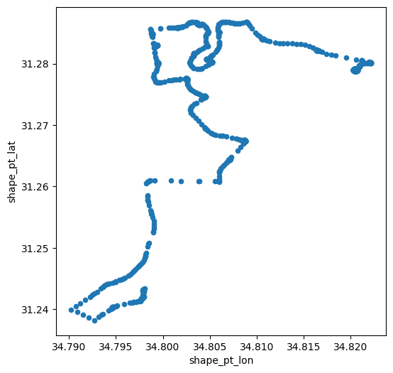
Fig. 32 Solution of exercise-06-f: Coordinates of the 1^st trip of bus '24' by 'דן באר שבע'

Exercise 06-g

• In this exercise, you are going to find the names of the five longest bus routes (in terms of distance traveled) in Israel. To do that, go through the following steps.

• Read the stop_times.txt table and select just the 'trip_id' and 'shape_dist_traveled' columns.

• Calculate the maximum (i.e., total) distance traveled ('shape_dist_traveled') for each public transit trip ('trip_id') (Fig. 33).

• Read the trips.txt table and select just the 'trip_id', and 'route_id'.

• Join the resulting trips table with the stop_times table from the previous step (using the common "trip_id" column), to get the 'route_id' value of each trip.

• Retain just one (the first) trip per 'route_id' (Fig. 34).

• Read the routes.txt table and subset the 'route_id', 'route_short_name', and 'route_long_name' columns.

• Join the resulting table with the trips table (using the common 'route_id' column), to get the 'route_short_name' and 'route_long_name' values of each route (Fig. 35).

• Sort the table according to 'shape_dist_traveled' (from largest to smallest), and print the first five rows (Fig. 36). Those are the longest-distance public transport routes in the GTFS dataset.

• Convert the 'route_long_name' values of the first five rows from the previous step, collect them into a list, and print the list, to see the full names of the routes. You can see that all five routes are from Haifa to Eilat or the other way around.

	trip_id	shape_dist_traveled
0	10004214_011023	11152.0
1	10004215_011023	11152.0
2	1001407_011023	15061.0
3	10015281_071023	21688.0
4	10015281_081023	21688.0
...	...	...
398086	9998411_091023	14147.0
398087	9998411_131023	14040.0
398088	9999194_061023	13597.0
398089	9999194_081023	13597.0
398090	9999194_151023	13597.0

398091 rows × 2 columns

Fig. 33 Solution of exercise-06-g: Total distance traveled in each trip, based on stop_times.txt

	route_id	trip_id	shape_dist_traveled
0	1	17336167_081023	7258.0
1	2	13076786_081023	7088.0
2	3	5655904_011023	9883.0
3	4	585026983_011023	7025.0
4	5	5656121_081023	9750.0
...	...	...	...
8183	37315	1_88437	NaN
8184	37316	1_88438	NaN
8185	37342	585305994_121023	16432.0
8186	37343	585305995_121023	16761.0
8187	37350	1_88086	NaN

8188 rows × 3 columns

Fig. 34 Solution of exercise-06-g: Joined with trips.txt, selecting just the 1^st trips per route_id

	route_id	route_short_name	route_long_name	trip_id	shape_dist_traveled
0	1	1	ת. רכבת יבנה מערב-יבנה<->ת. רכב...	17336167_081023	7258.0
1	2	1	ת. רכבת יבנה מזרח-יבנה<->ת. רכב...	13076786_081023	7088.0
2	3	2	ת. רכבת יבנה מערב-יבנה<->ת. רכב...	5655904_011023	9883.0
3	4	2א	ת. רכבת יבנה מערב-יבנה<->ת. רכב...	585026983_011023	7025.0
4	5	2	ת. רכבת יבנה מזרח-יבנה<->ת. רכב...	5656121_081023	9750.0
...	...	...	...	...	...
8183	37315	NaN	תא אוניברסיטה-תל אביב יפו<->באר...	1_88437	NaN
8184	37316	NaN	תא אוניברסיטה-תל אביב יפו<->הרצ...	1_88438	NaN
8185	37342	46	גן טכנולוגי-נצרת<->מסרארה חט''ב...	585305994_121023	16432.0
8186	37343	46	גן טכנולוגי-נצרת<->מסרארה חט''ב...	585305995_121023	16761.0
8187	37350	NaN	באר שבע מרכז-באר שבע<->נהריה-נהריה	1_88086	NaN

8188 rows × 5 columns

Fig. 35 Solution of exercise-06-g: Joined with routes.txt

	route_id	route_short_name	route_long_name	trip_id	shape_dist_traveled
5155	19964	991	ת. מרכזית חוף הכרמל/רציפים בינע...	30526427_091023	446163.0
5475	21726	991	ת. מרכזית אילת/רציפים-אילת<->ת....	30526417_061023	445475.0
1456	7307	993	ת. מרכזית המפרץ/רציפים בינעירונ...	2125973_151023	432200.0
1455	7305	993	ת. מרכזית אילת/רציפים-אילת<->ת....	584673295_011023	432187.0
1153	5182	399	ת. מרכזית חדרה/רציפים-חדרה<->ת....	584660100_091023	401875.0

Fig. 36 Solution of exercise-06-g: Sorted by shape_dist_traveled, from largest to smallest

Exercise solutions

Exercise 06-b

import numpy as np
import pandas as pd
# Read data
dat = pd.read_csv('data/ZonAnn.Ts+dSST.csv')
cols = ['90S-64S', '64S-44S', '44S-24S', '24S-EQU', 'EQU-24N', '24N-44N', '44N-64N', '64N-90N']
regions = dat[cols]
# Function to calculate linear slope
def f(x, y): 
    return np.polyfit(x, y, 1)[0]
f(dat['Year'], regions['44S-24S'])

np.float64(0.006830158347399733)

# Calculate slopes per region
regions.apply(lambda i: f(dat['Year'], i), axis=0)

90S-64S    0.006262
64S-44S    0.005188
44S-24S    0.006830
24S-EQU    0.006690
EQU-24N    0.006562
24N-44N    0.008564
44N-64N    0.012204
64N-90N    0.018884
dtype: float64

Exercise 06-d

import pandas as pd
# Read
routes = pd.read_csv('data/gtfs/routes.txt')
trips = pd.read_csv('data/gtfs/trips.txt')
# Join
dat = pd.merge(trips, routes, on='route_id', how='left')
# Calculate number of unique trips per route
dat = dat.groupby(['route_id', 'route_short_name', 'route_long_name']).nunique()['trip_id'].reset_index()
# Sort
dat = dat.sort_values('trip_id', ascending=False)
dat

Exercise 06-e

import pandas as pd
trips = pd.read_csv('data/gtfs/trips.txt')
trips.groupby('route_id')['shape_id'].nunique().value_counts().sort_index()

Exercise 06-f

import pandas as pd
# Read
agency = pd.read_csv('data/gtfs/agency.txt')
routes = pd.read_csv('data/gtfs/routes.txt')
trips = pd.read_csv('data/gtfs/trips.txt')
shapes = pd.read_csv('data/gtfs/shapes.txt')
# Subset
agency = agency[['agency_id', 'agency_name']]
routes = routes[['route_id', 'agency_id', 'route_short_name', 'route_long_name']]
trips = trips[['trip_id', 'route_id', 'shape_id']]
shapes = shapes[['shape_id', 'shape_pt_sequence', 'shape_pt_lon', 'shape_pt_lat']]
# Filter agency
agency = agency[agency['agency_name'] == 'דן באר שבע']
routes = routes[routes['agency_id'] == agency['agency_id'].iloc[0]]
routes = routes.drop('agency_id', axis=1)
# Filter route
routes = routes[routes['route_short_name'] == '24']
# Filter trip
routes = pd.merge(routes, trips, on='route_id', how='left')
trip = routes[routes['trip_id'] == routes['trip_id'].iloc[0]]
# Join with 'shapes'
trip = pd.merge(trip, shapes, on='shape_id', how='left')
trip = trip.sort_values(by='shape_pt_sequence')
trip

	route_id	route_short_name	route_long_name	trip_id	shape_id	shape_pt_sequence	shape_pt_lon	shape_pt_lat
0	17537	24	ת.מרכזית/עירוניים לצפון-באר שבע...	26385618_011023	136236.0	1	34.797979	31.242009
1	17537	24	ת.מרכזית/עירוניים לצפון-באר שבע...	26385618_011023	136236.0	2	34.797988	31.242103
2	17537	24	ת.מרכזית/עירוניים לצפון-באר שבע...	26385618_011023	136236.0	3	34.797982	31.242829
3	17537	24	ת.מרכזית/עירוניים לצפון-באר שבע...	26385618_011023	136236.0	4	34.797986	31.242980
4	17537	24	ת.מרכזית/עירוניים לצפון-באר שבע...	26385618_011023	136236.0	5	34.798000	31.243121
...	...	...	...	...	...	...	...	...
856	17537	24	ת.מרכזית/עירוניים לצפון-באר שבע...	26385618_011023	136236.0	857	34.822166	31.280183
857	17537	24	ת.מרכזית/עירוניים לצפון-באר שבע...	26385618_011023	136236.0	858	34.822116	31.280225
858	17537	24	ת.מרכזית/עירוניים לצפון-באר שבע...	26385618_011023	136236.0	859	34.822038	31.280246
859	17537	24	ת.מרכזית/עירוניים לצפון-באר שבע...	26385618_011023	136236.0	860	34.821949	31.280250
860	17537	24	ת.מרכזית/עירוניים לצפון-באר שבע...	26385618_011023	136236.0	861	34.821860	31.280233

861 rows × 8 columns

trip.plot.scatter(x='shape_pt_lon', y='shape_pt_lat');

Exercise 06-g

import pandas as pd
# Get total distance traveled per 'trip_id'
stop_times = pd.read_csv('data/gtfs/stop_times.txt')
stop_times = stop_times.groupby('trip_id')['shape_dist_traveled'].max()
stop_times = stop_times.reset_index()
stop_times

	trip_id	shape_dist_traveled
0	10004214_011023	11152.0
1	10004215_011023	11152.0
2	1001407_011023	15061.0
3	10015281_071023	21688.0
4	10015281_081023	21688.0
...	...	...
398086	9998411_091023	14147.0
398087	9998411_131023	14040.0
398088	9999194_061023	13597.0
398089	9999194_081023	13597.0
398090	9999194_151023	13597.0

398091 rows × 2 columns

# Join with trips to get 'route_id' per trip
trips = pd.read_csv('data/gtfs/trips.txt')
trips = trips[['trip_id', 'route_id']]
trips = pd.merge(trips, stop_times, on='trip_id')
trips = trips.groupby('route_id').first()
trips = trips.reset_index()
trips

	route_id	trip_id	shape_dist_traveled
0	1	17336167_081023	7258.0
1	2	13076786_081023	7088.0
2	3	5655904_011023	9883.0
3	4	585026983_011023	7025.0
4	5	5656121_081023	9750.0
...	...	...	...
8183	37315	1_88437	NaN
8184	37316	1_88438	NaN
8185	37342	585305994_121023	16432.0
8186	37343	585305995_121023	16761.0
8187	37350	1_88086	NaN

8188 rows × 3 columns

# Join with routes to get route short/long names
routes = pd.read_csv('data/gtfs/routes.txt')
routes = routes[['route_id', 'route_short_name', 'route_long_name']]
routes = pd.merge(routes, trips, on='route_id')
routes

	route_id	route_short_name	route_long_name	trip_id	shape_dist_traveled
0	1	1	ת. רכבת יבנה מערב-יבנה<->ת. רכב...	17336167_081023	7258.0
1	2	1	ת. רכבת יבנה מזרח-יבנה<->ת. רכב...	13076786_081023	7088.0
2	3	2	ת. רכבת יבנה מערב-יבנה<->ת. רכב...	5655904_011023	9883.0
3	4	2א	ת. רכבת יבנה מערב-יבנה<->ת. רכב...	585026983_011023	7025.0
4	5	2	ת. רכבת יבנה מזרח-יבנה<->ת. רכב...	5656121_081023	9750.0
...	...	...	...	...	...
8183	37315	NaN	תא אוניברסיטה-תל אביב יפו<->באר...	1_88437	NaN
8184	37316	NaN	תא אוניברסיטה-תל אביב יפו<->הרצ...	1_88438	NaN
8185	37342	46	גן טכנולוגי-נצרת<->מסרארה חט''ב...	585305994_121023	16432.0
8186	37343	46	גן טכנולוגי-נצרת<->מסרארה חט''ב...	585305995_121023	16761.0
8187	37350	NaN	באר שבע מרכז-באר שבע<->נהריה-נהריה	1_88086	NaN

8188 rows × 5 columns

# Sort accordinge to distance traveled
routes = routes.sort_values('shape_dist_traveled', ascending=False).head()
routes

	route_id	route_short_name	route_long_name	trip_id	shape_dist_traveled
5155	19964	991	ת. מרכזית חוף הכרמל/רציפים בינע...	30526427_091023	446163.0
5475	21726	991	ת. מרכזית אילת/רציפים-אילת<->ת....	30526417_061023	445475.0
1456	7307	993	ת. מרכזית המפרץ/רציפים בינעירונ...	2125973_151023	432200.0
1455	7305	993	ת. מרכזית אילת/רציפים-אילת<->ת....	584673295_011023	432187.0
1153	5182	399	ת. מרכזית חדרה/רציפים-חדרה<->ת....	584660100_091023	401875.0

routes.head()["route_long_name"].to_list()

['ת. מרכזית חוף הכרמל/רציפים בינעירוני-חיפה<->ת. מרכזית אילת/הורדה-אילת-2#',
 'ת. מרכזית אילת/רציפים-אילת<->ת. מרכזית חוף הכרמל/הורדה-חיפה-1#',
 'ת. מרכזית המפרץ/רציפים בינעירוני-חיפה<->ת. מרכזית אילת/הורדה-אילת-2#',
 'ת. מרכזית אילת/רציפים-אילת<->ת. מרכזית המפרץ/הורדה-חיפה-1#',
 'ת. מרכזית חדרה/רציפים-חדרה<->ת. מרכזית אילת/הורדה-אילת-1#']

---

[1]

For a visual explanation of join types, see https://dataschool.com/how-to-teach-people-sql/sql-join-types-explained-visually/.