ArcGIS Pro scripting (arcpy)

ArcGIS Pro scripting (`arcpy`)#

Last updated: 2024-03-03 15:41:43

Introduction#

So far, we worked with Python as a standalone program, utilizing both the standard library and third-party packages. In addition to this mode of operation, the Python language is often used to automate other programs. For example, when working with a GUI (Graphical User Interface) GIS software, such as ArcGIS Pro or QGIS, it can be exhausting and non-reproducible to perform repetitive tasks and workfows. It is advantageous to write-up such workflows as Python scripts, so that they can be easily reproduced for different data or shared with colleagues.

Automating workflows within GIS software, such as ArcGIS Pro or QGIS, is made possible through their accompanying Python packages, arcpy and PyQGIS, respectively. As we are going to see in this chapter, the specialized Python packages such as arcpy provide access to the entire functionality of the program, including the various data management and processing tools, so that a particular workflow can be described in a reproducible Python script.

GIS software automation vs. standalone Python#

In this Chapter, we introduce the ability to automate ArcGIS Pro geoprocessing tools by writing Python code. This is an alternative pathway to achieve much of the same capabilities covered in previous chapters. What are, then, the advantages and disadvantages of the two approaches, and when should we prefer one or the other?

Advantages of geoprocessing through standalone Python scripts, using packages such as geopandas and rasterio, are:

Python and the third-party packages are free and open-source, making the workflow independent and reproducible (unlike ArcGIS Pro which is paid software)
The code for most tasks is often more simple, more similar to other software (rather than specialized), and not restricted to ArcGIS Pro functions

Advantages of scripts to automate the ArcGIS Pro software through the arcpy Python package, are:

Sharing the script with other people who are familiar with ArcGIS Pro (but not Python) is easy
ArcGIS Pro provides a wide range of geoprocessing functions, some of them not found at all, or complicated to use, in open-source tools, such as 3D analysis

To summarize, it is advantageous to use arcpy when you are already well familiar with the software and/or work with its specialized functionality not found elsewhere.

Python interfaces in ArcGIS Pro#

ArcGIS Pro has two main interfaces for running Python code (Fig. 73):

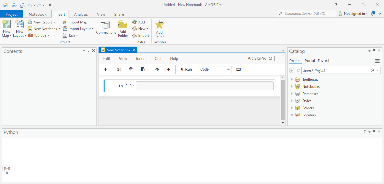
_images/arcpro_notebook.png — Fig. 73 Python console and Jupyter notebook in ArcGIS Pro#

To start the Python window or open a Jupyter notebook, go to the Analysis tab, then click on the Python button (in the Geoprocessing group) and select either the Python Notebook option or the Python window option. To open a Jupyter notebook, you can also go to the Insert tab, then click on the New Notebook button (in the Project group).

The Python window and the Jupyter notebook interfaces are analogous to a standalone Python console and a standalone Jupyter notebook, which we are familiar with (see The Python command line and Jupyter Notebook). The difference is that:

The ArcGIS Pro Python window and notebooks interfaces are embedded in the ArcGIS Pro program, so they need to be started when running ArcGIS Pro
The ArcGIS Pro Python interfaces include the pre-installed arcpy package, which is an interface to ArcGIS Pro geoprocessing tools through Python

Just like their standalone versions, the ArcGIS Pro Python window is often useful for experimenting with Python expressions or short scripts, while notebooks are suitable for developing longer scripts associated with textual comments.

You can run the code examples in this chapter either in a Jupyter notebook or in a Python window in ArcGIS Pro. Note that when pasting a multi-line code block into the Python window, you need to press Ctrl+Enter to execute it.

What is `arcpy`?#

arcpy is a Python package that provides an interface to the entire functionality of the ArcGIS Pro software. Therefore, arcpy can be used to:

Document ArcGIS Pro workflows, thus making them reproducible
Automate repetitive tasks that are unfeasible or work-intensive in the ArcGIS Pro GUI

Note

See the A quick tour of ArcPy help page for an overview of arcpy.

Importing layers#

The following code section can be used to load a Shapefile on the ArcGIS Pro map, using Python:

import arcpy
aprx = arcpy.mp.ArcGISProject('CURRENT')
map = aprx.listMaps()[0]
map.addDataFromPath('C:/Users/dorman/Downloads/data/RAIL_STAT_ONOFF_MONTH.shp')

Let’s go over the meaning of the five expressions:

import arcpy—Loads the arcpy package, making it possible to interact with the ArcGIS Pro software
aprx=...—Creates a reference to the ArcGIS Pro project we intend to interact with (in this case, the 'CURRENT' project)
map=...—Creates a reference to the map we intend to interact with, within the project (in this case, the first map, 0).
map.addDataFromPath('...')—Adds the Shapefile located at the specified file path to the map

Note that the project must have a map open for the code to work! To open a map, go to the Insert tab, then click on the New Map button (in the Project group). Also make sure to modify the Shapefile path according to the path of the Shapefile you are going to load. In this example, the Shapefile we load is the railway station layer which we are already familiar with (see Railway stations). If all worked well, you should see the railway stations layer in the table of contents as well as on the map (Fig. 74).

_images/arcpy_import_layer.png — Fig. 74 The railway station layer (`'RAIL_STAT_ONOFF_MONTH.shp'`) imported using `arcpy`#

Remember that the Python code sections in this chapter cannot be run in the usual Jupyter Notebook environment which we have been using until now, because they require the arcpy library which connects to an ArcGIS Pro installation. Therefore, the code sections must be run in one of the ArcGIS Pro Python interfaces: the Python window or a ArcGIS Pro Jupyter Notebook (see Python interfaces in ArcGIS Pro).

Note

See the Map class documentation for more details about working with maps in arcpy.

Using geoprocessing functions#

Overview#

Once the layers we are working with are imported into ArcGIS Pro, writing a geoprocessing script is mostly a matter of locating the right ArcGIS Pro function(s) and their required parameters. The arcpy package gives access to the wide variety of geoprocessing tools in the ArcGIS Pro software. Finding the right functions will be easier for those who are already familiar with ArcGIS Pro, because arcpy is essentially a command-line interface to exactly the same “ordinary” ArcGIS Pro tools, which are accessible through buttons and dialog boxes. Accordingly, help pages of geoprocessing tools provide side-to-side documentation on how to use the tool through a dialog box and through arcpy (Fig. 75).

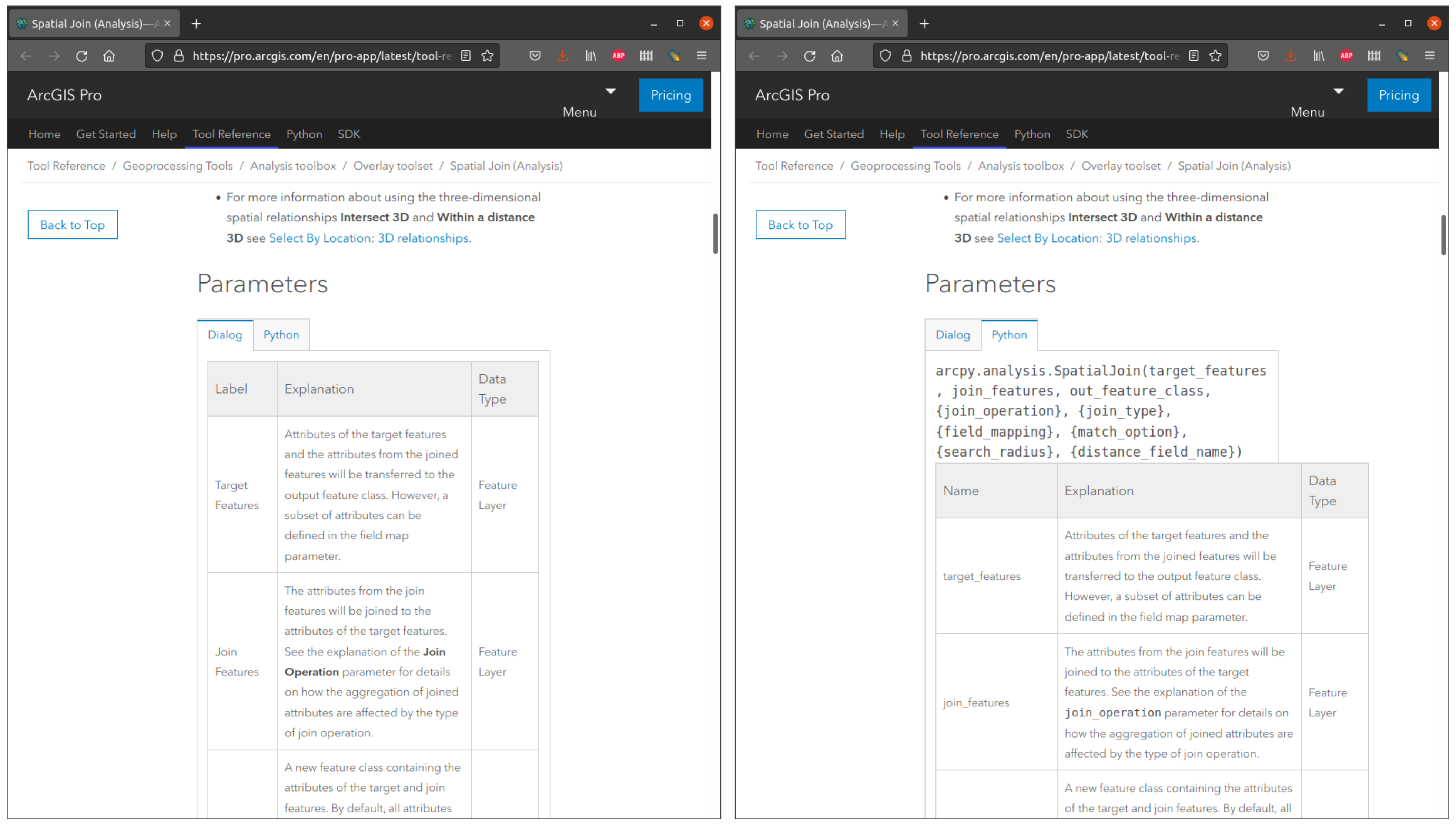
_images/arcpy_docs.png — Fig. 75 The help page for the spatial join tool in ArcGIS Pro, with side-by-side documentation on how to run the tool through a dialog box (left) and through a Python script using `arcpy` function `arcpy.analysis.SpatialJoin` (right).#

In the following two sections, we demonstrate two geoprocessing tasks with arcpy:

Buffers (arcpy)
Subsetting by attributes (arcpy)

Buffers (`arcpy`)#

To calculate buffers (see Buffers (geopandas)), for example, we can use the arcpy.analysis.Buffer function. Let us calculate a buffer around the railway station points. The first three and most important parameters of arcpy.analysis.Buffer are:

in_features—The input layer
out_feature_class—The name of the output buffered layer
buffer_distance_or_field—The buffer distance(s), either a numeric/text value, or the name of an attribute

For example, the following expression buffers the railway station point layer to a distance of 1000 meters, creating a new polygon layer named RAIL_STAT_ONOFF_MONTH_1000:

arcpy.analysis.Buffer(
    'RAIL_STAT_ONOFF_MONTH', 
    'RAIL_STAT_ONOFF_MONTH_1000', 
    '1000 meters'
)

The new layer also appears on the map in ArcGIS Pro (Fig. 76).

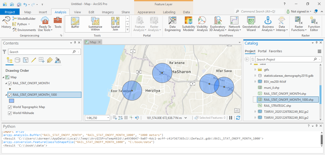
_images/arcpy_buffer_export.png — Fig. 76 Calculting a buffer and exporting using the Python console#

Subsetting by attributes (`arcpy`)#

To demonstrate subsetting by attributes (see Filtering by attributes), let’s also import the Shapefile named 'RAIL_STRATEGIC.shp', which contains railway lines. To do that, we are using map.addDataFromPath the same way we did for importing the railway stations layer (see Importing layers):

map.addDataFromPath('C:/Users/dorman/Downloads/data/RAIL_STRATEGIC.shp')

To subset the features of interest, we can use a combination of arcpy.management.SelectLayerByAttribute and arcpy.management.CopyFeatures. If you are familiar with GIS software, you may notice this replicates the usual workflow where the features of interest are first selected (thus “highlighted” in the attribute table and on the map), and then the active selection is exported to a new layer:

arcpy.management.SelectLayerByAttribute(
    'RAIL_STRATEGIC', 
    'NEW_SELECTION', 
    '"ISACTIVE" = \'פעיל\''
)
arcpy.management.CopyFeatures('RAIL_STRATEGIC', 'RAIL_STRATEGIC_active')

Note the 'NEW_SELECTION' argument in arcpy.management.SelectLayerByAttribute, which specified that the selection starts from scratch (rather than, for instance, adding to an existing selection). The next argument is a string with a conditional expression, specifying which features to select, namely "ISACTIVE" = \'פעיל\'". Finally, the arcpy.management.CopyFeatures function is used to make a copy of the layer. Importantly, if there is any selection on the input layer then only the selected features are copied to the output layer.

Accessing data#

arcpy provides several methods of accessing the attribute table values, for example, to export them or to calculate new attributes. Since we are already familiar with numpy, we will demonstrate the arcpy.da.TableToNumPyArray function, which exports the attributes to a numpy array.

The arcpy.da.TableToNumPyArray function takes two arguments:

The layer name
The name(s) of the attribute(s) to extract

The returned object is a numpy array.

For example, the following expression extracts the attributes 'ON_7_DAY' and 'OFF_7_DAY' (number of passengers entering and exiting the station, respectively, at 7:00-8:00), from the RAIL_STAT_ONOFF_MONTH layer, to an array named dat:

dat = arcpy.da.TableToNumPyArray('RAIL_STAT_ONOFF_MONTH', ['ON_7_DAY', 'OFF_7_DAY'])

The result is a special type of array, called a structured array. A structured array is an array where each element is a combination of several named values. In our case, the array is composed of pairs of values ('ON_7_DAY', and 'OFF_7_DAY'), both of type float64. Individual components can be accessed by name, as in:

dat['ON_7_DAY']
dat['OFF_7_DAY']

Each of the above expressions returns an “ordinary” one-dimensional array (Fig. 77).

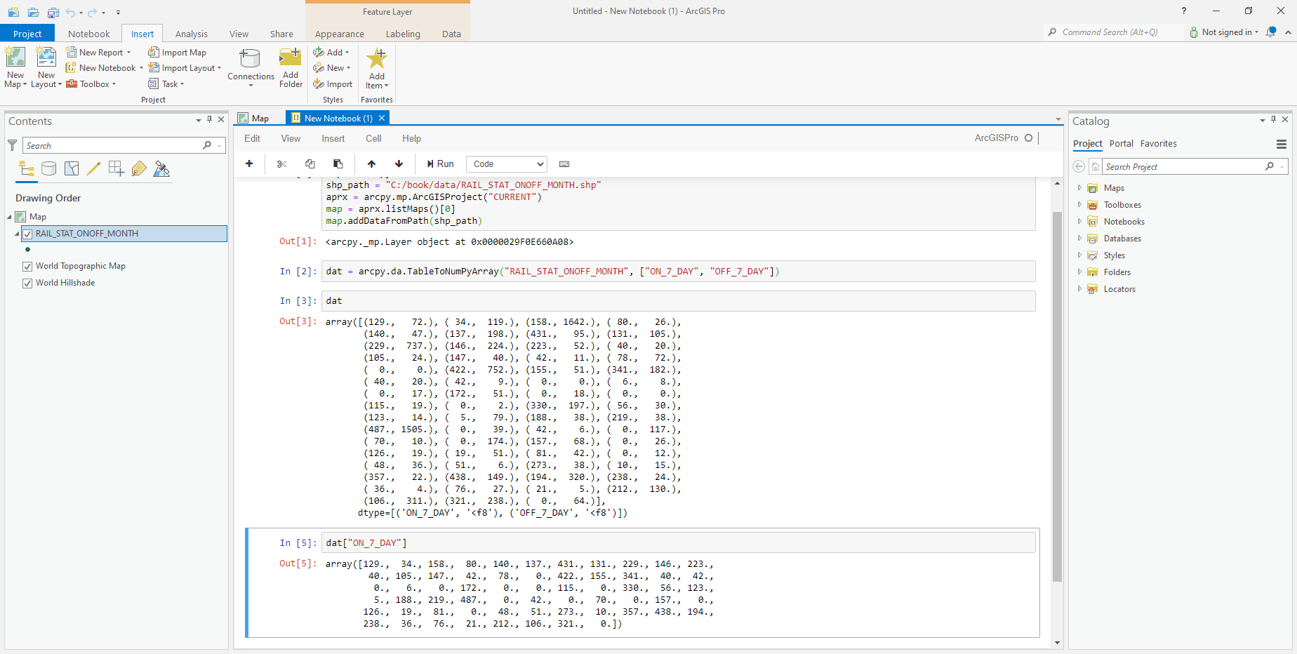
_images/arcpy_structured_array.png — Fig. 77 Structured array with the `'ON_7_DAY'` and `'OFF_7_DAY'` attribute values extracted from the `RAIL_STAT_ONOFF_MONTH` layer#

Modifying data#

The arcpy.da.UpdateCursor function can be used to iterate over rows in a layer, and to modify them. The arcpy.da.UpdateCursor function is basically a method to access a subset of attributes as an iterable object. Then, we can go over the rows, doing something with the attribute(s) in that row. For example, suppose that we would like to calculate a new column named 'sum_7_day', which is the sum of passengers entering and exiting the station at 7 AM, i.e., the sum of the 'ON_7_DAY' and 'OFF_7_DAY' attributes. The calculation of the new 'sum_7_day' column takes two steps.

First, we create a new column named 'sum_7_day', of type 'Double' (i.e., numeric). This column is going to accomodate the sums of the 'ON_7_DAY' and 'OFF_7_DAY' attributes:

arcpy.AddField_management('RAIL_STAT_ONOFF_MONTH', 'sum_7_day', 'Double')

Second, we access the layer with the arcpy.da.UpdateCursor function, creating a “cursor” object named cursor. When initializing the cursor object, we also pass a list of column names that we are going to work with: ['ON_7_DAY', 'OFF_7_DAY', 'sum_7_day'].

Inside the cursor context, we iterate over the rows using a for loop. Note that this is similar to the way that we used a for loop to iterate over a “reader” object when reading a CSV file (Reading CSV files). In the iteration, row is a list of values in the specified order of columns. For each row, we are summing the 'ON_7_DAY', 'OFF_7_DAY' values in that given row, using row[0]+row[1], and then assigning the result to the 'sum_7_day' value, using row[2]=.... The last expression cursor.updateRow(row) makes sure that the modified row is updated in the layer itself. Finally, we “reset” the cursor with cursor.reset():

cursor = arcpy.da.UpdateCursor(
    in_table='RAIL_STAT_ONOFF_MONTH', 
    field_names=['ON_7_DAY', 'OFF_7_DAY', 'sum_7_day']
)
for row in cursor:
    row[2] = row[0] + row[1]
    cursor.updateRow(row)
cursor.reset()

As a result, the attribute table of the 'RAIL_STAT_ONOFF_MONTH' layer now contains the new attribute named 'sum_7_day' (Fig. 78).

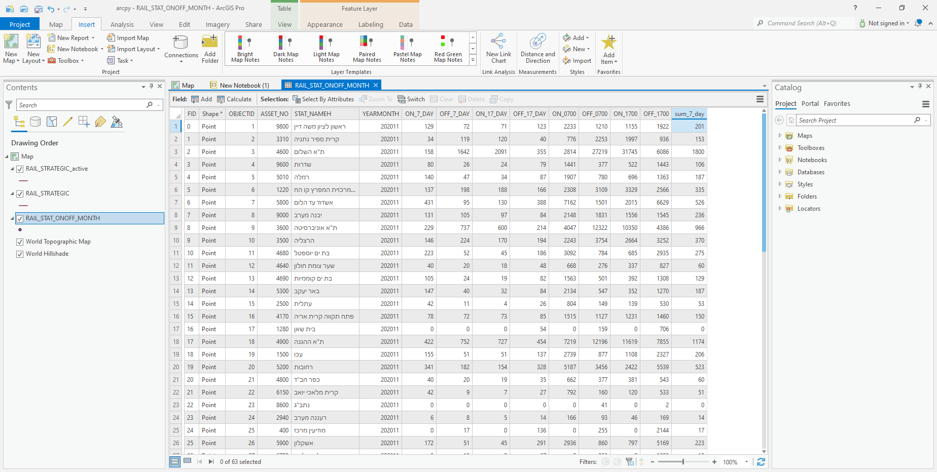
_images/arcpy_cursor.png — Fig. 78 New attribute `'sum_7_day'` calculated in the `'RAIL_STAT_ONOFF_MONTH'` layer#

Nearest neighbor join (`arcpy`)#

The arcpy.SpatialJoin_analysis function can be used for spatial join. Notably, the arcpy.SpatialJoin_analysis function has a wide range of options to specify the conditions to find “matching” features, and methods to summarize multiple matches into a single attribute value (e.g., mean or median of all matches). For example, there is a “nearest neighbor” join option, similar in scope to the gpd.sjoin_nearest function from geopandas (see Nearest neighbor join).

The following expression finds the nearest railway segment (from 'RAIL_STRATEGIC_active') for each railway station ('RAIL_STAT_ONOFF_MONTH'), then attaches that segment attributes and its distance to the station into the attribute table of 'RAIL_STAT_ONOFF_MONTH':

arcpy.SpatialJoin_analysis(
    'RAIL_STAT_ONOFF_MONTH', 
    'RAIL_STRATEGIC_active', 
    'join_output', 
    match_option = 'CLOSEST',
    distance_field_name = 'dist'
)

Fig. 79 shows the attribute table of the resulting layer join_output. Note that the attribute table contains the attributes of the nearest railway line segment (such as 'SEGMENT', i.e., segment name) for each railway station feature.

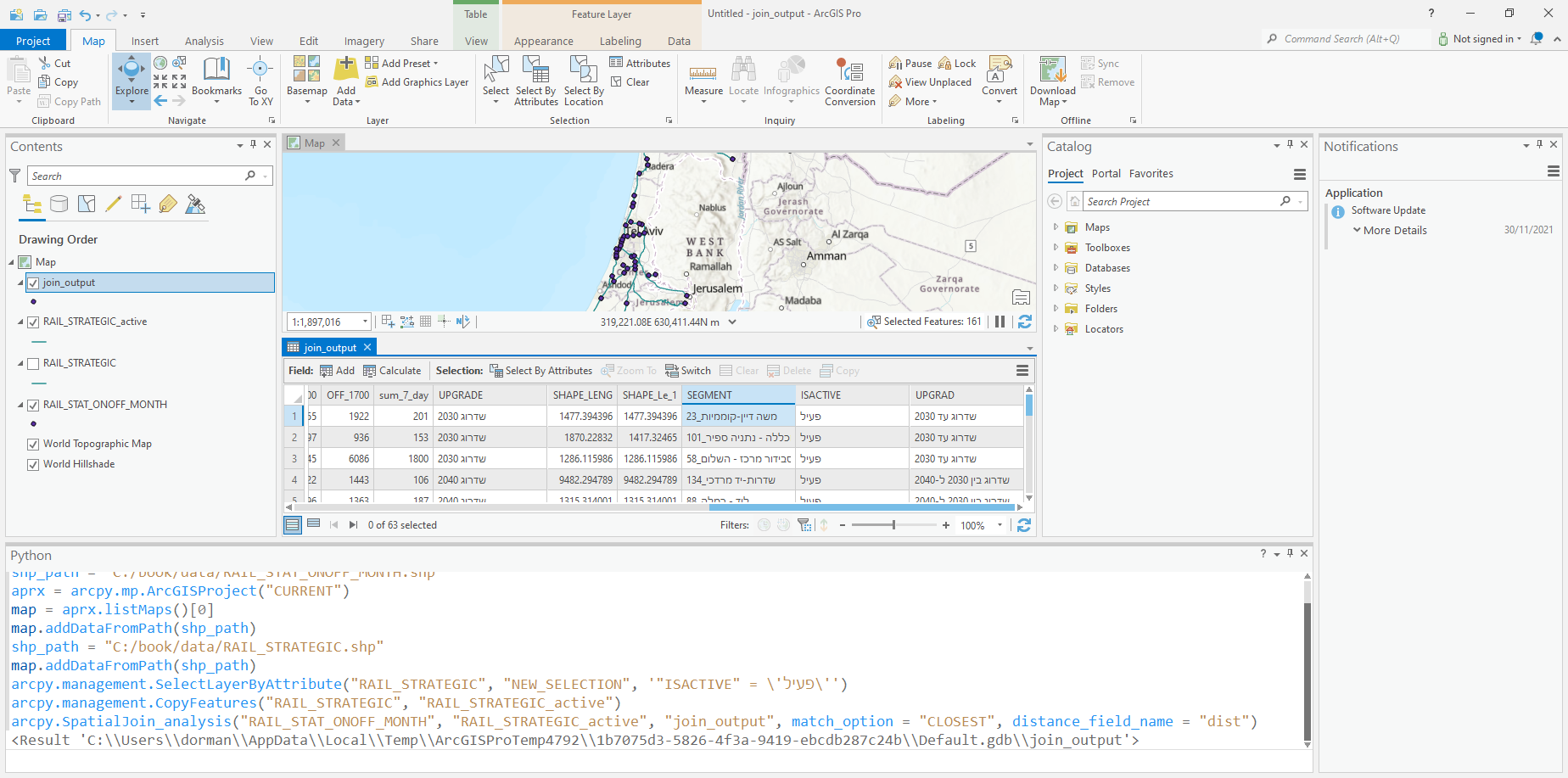
_images/arcpy_join_output.png — Fig. 79 Attribute table of nearest neighbor join output `'join_output'`, containing the attributes of nearest railway segment for each railway station#

Exporting results#

A “layer” in the ArcGIS Pro environment, such as the 'join_output' layer we have just created (see Nearest neighbor join (arcpy)), is an abstract structure which only makes sense inside the ArcGIS Pro environment. For permanently storing a layer, whether for future analysis or for sharing with other people, we need to export the layer into a file, such as a Shapefile.

The arcpy.conversion.FeatureClassToShapefile can be used to export a layer we created as a Shapefile. For example, here is how we can export the 'RAIL_STAT_ONOFF_MONTH_1000' (railway station buffers) and the 'join_output' (railway stations joined with nearest railway line attributes) to Shapefiles:

arcpy.conversion.FeatureClassToShapefile(
    'RAIL_STAT_ONOFF_MONTH_1000', 
    'C:/Users/dorman/Downloads/output/'
)
arcpy.conversion.FeatureClassToShapefile(
    'join_output', 
    'C:/Users/dorman/Downloads/output/'
)

Exercises#

Exercise 12-a

Create a point layer from the 'stops.txt' file in the GTFS dataset (Fig. 80).
Hint: use the arcpy.conversion.GTFSStopsToFeatures function.

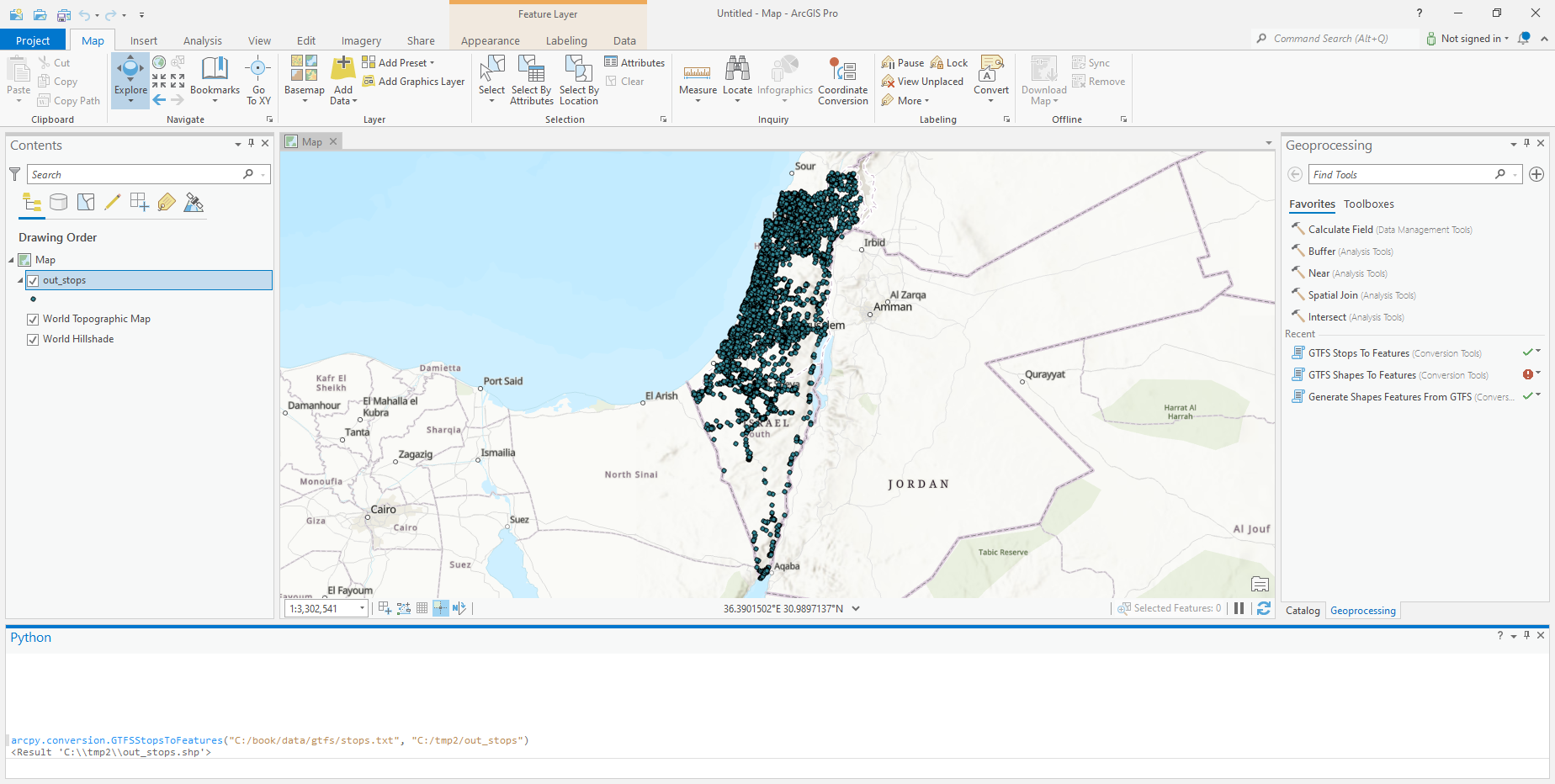
_images/arcpy_gtfs_stops.png — Fig. 80 Point layer generated from the `'stops.txt'` file in a GTFS dataset#

Exercise 12-b

Create a layer of Haifa statistical areas with an attribute of average elevation, recreating the rasterstats-based calculation (see Zonal statistics).
Hint: check out the Zonal Statistics as Table (Spatial Analyst) documentation.

Exercise solutions#

Exercise 11-a#

import arcpy
arcpy.conversion.GTFSStopsToFeatures(
    'C:/Users/dorman/Downloads/data/gtfs/stops.txt', 
    'C:/Users/dorman/Downloads/output/out_stops'
)

Exercise 11-b#

import arcpy

# Add polygons
arcpy.management.MakeFeatureLayer(
    'C:/book/data/statisticalareas_demography2019.gdb/statisticalareas_demography2019', 
    'stat'
)

# Add raster
arcpy.MakeRasterLayer_management(
    'C:/Users/dorman/Downloads/output/carmel.tif', 
    'carmel.tif'
)

# Subset
arcpy.management.SelectLayerByAttribute(
    'stat', 
    'NEW_SELECTION', 
    '"SHEM_YISHUV" = \'חיפה\''
)
arcpy.management.CopyFeatures('stat', 'stat2')

# Extract
arcpy.sa.ZonalStatisticsAsTable(
    'stat2', 
    'STAT11', 
    'carmel.tif', 
    'C:/Users/dorman/Downloads/output/out.dbf', 
    'DATA', 
    'MEAN'
)

# Join table with polygons
arcpy.AddJoin_management('stat2', 'STAT11', 'out', 'STAT1')

# Write
arcpy.conversion.FeatureClassToShapefile('stat2', 'C:/Users/dorman/Downloads/output/')

# Copy the layer to a new permanent feature class
arcpy.CopyFeatures_management(veg_joined_table, outFeature)