
Geometric operations#
Last updated: 2025-01-15 17:43:32
Introduction#
In the previous chapter we introduced the geopandas package, focusing on non-spatial operations such as subsetting by attributes (see Filtering by attributes), as well as geometry-related transformations (see Table to point layer and Points to line (geopandas)).
In this chapter, we go further into operations that involve the geometric component of one or more GeoDataFrames, using the geopandas package. This group of operations includes the following standard spatial analysis functions:
CRS and reprojection—Transforming a given layer from one CRS to another
Numeric calculations—Calculating numeric geometry properties, such as length, area, and distance
New geometries 1 (geopandas), New geometries 2 (geopandas)—Creating new geometries, such as calculating buffers, or areas of intersection
Boolean methods (geopandas)—Evaluating the relation between layers, such as whether their geometries intersect
Spatial join—Joining attributes from one layer to another, based on spatial relations
By the end of this chapter, you will have an overview of all common worflows in spatial analysis of vector layers.
Sample data#
Overview#
First, let’s prepare the environment to demostrate geometric operations using geopandas. First, we load the pandas and geopandas packages:
import pandas as pd
import geopandas as gpd
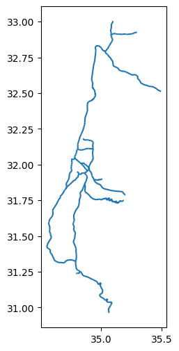
Next, let’s load three layers, subset the relevant columns, and examine them visually. The first two (towns and rail) are familiar from the previous chapter (see Reading vector layers), while the third one (stations) is new:
towns—A polygonal layer of towns (see Towns)rail—A line layer of railway lines (see Railway lines)stations—A point layer of railway stations (see Railway stations)
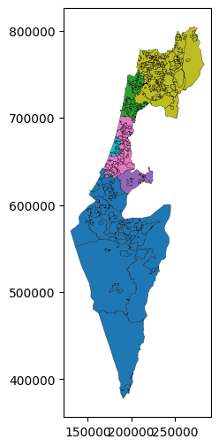
Towns#
The polygonal towns layer is imported from the Shapefile named 'muni_il.shp'. Then we select the attributes of interest, plus the 'geometry' column:
towns = gpd.read_file('data/muni_il.shp', encoding='utf-8')
towns = towns[['Muni_Heb', 'Machoz', 'Shape_Area', 'geometry']]
towns
| Muni_Heb | Machoz | Shape_Area | geometry | |
|---|---|---|---|---|
| 0 | שפיר | דרום | 2.721176e+07 | POLYGON Z ((177281.694 610056.5... |
| 1 | דימונה | דרום | 7.708050e+04 | POLYGON Z ((205753.745 560693.6... |
| 2 | דימונה | דרום | 1.043253e+06 | POLYGON Z ((207740.171 563476.5... |
| 3 | זבולון | חיפה | 4.769053e+04 | POLYGON Z ((209445.229 740507.2... |
| 4 | מגידו | צפון | 2.144091e+04 | POLYGON Z ((206769.626 727131.7... |
| ... | ... | ... | ... | ... |
| 406 | ללא שיפוט - אזור מעיליא | צפון | 2.001376e+05 | POLYGON Z ((225369.655 770523.6... |
| 407 | זבולון | חיפה | 2.246316e+05 | POLYGON Z ((207596.214 746263.0... |
| 408 | זבולון | חיפה | 1.141930e+06 | POLYGON Z ((208622.688 746540.1... |
| 409 | רמת השרון | תל אביב | 4.076764e+04 | POLYGON Z ((183576.756 673627.0... |
| 410 | צור הדסה | ירושלים | 3.961142e+06 | POLYGON Z ((209871.005 625364.9... |
411 rows × 4 columns
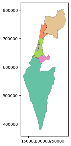
Here is the towns layer, colored by the 'Machoz' administrative division:
towns.plot(column='Machoz', edgecolor='black', linewidth=0.2);
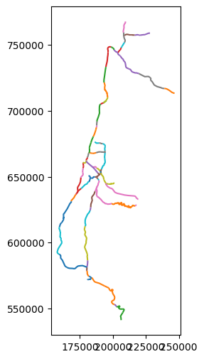
Railway lines#
Next, we read the railway line layer, from the Shapefile named 'RAIL_STRATEGIC.shp'. We subset the layer by attributes (see Filtering by attributes) to retain just the active railway segments. Then, we subset just the 'SEGMENT' (segment name) and 'geometry' columns:
rail = gpd.read_file('data/RAIL_STRATEGIC.shp')
rail = rail[rail['ISACTIVE'] == 'פעיל']
rail = rail[['SEGMENT', 'geometry']]
rail
| SEGMENT | geometry | |
|---|---|---|
| 0 | כפר יהושע - נשר_1 | LINESTRING (205530.083 741562.9... |
| 1 | באר יעקב-ראשונים_2 | LINESTRING (181507.598 650706.1... |
| 3 | לב המפרץ מזרח - נשר_4 | LINESTRING (203482.789 744181.5... |
| 4 | קרית גת - להבים_5 | LINESTRING (178574.101 609392.9... |
| 5 | רמלה - רמלה מזרח_6 | LINESTRING (189266.58 647211.50... |
| ... | ... | ... |
| 210 | ויתקין - חדרה_215 | LINESTRING (190758.23 704950.04... |
| 211 | בית יהושע - נתניה ספיר_216 | LINESTRING (187526.597 687360.3... |
| 214 | השמונה - בית המכס_220 | LINESTRING (200874.999 746209.3... |
| 215 | לב המפרץ - בית המכס_221 | LINESTRING (203769.786 744358.6... |
| 216 | 224_לוד מרכז - נתבג | LINESTRING (190553.481 654170.3... |
161 rows × 2 columns
Here is a plot of the rail layer, colored by segment name:
rail.plot(column='SEGMENT');
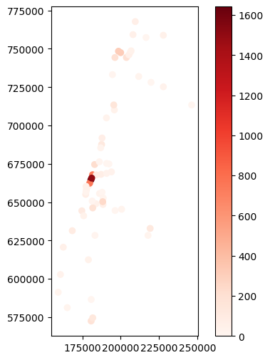
Railway stations#
Finally, we read a layer of rainway stations, from a Shapefile named 'RAIL_STAT_ONOFF_MONTH.shp'. The attributes of interest which we retain (in addition to the 'geometry') are:
'STAT_NAMEH'—Station name'OFF_7_DAY'—Passengers exiting the station at 7:00-8:00 during September 2020
stations = gpd.read_file('data/RAIL_STAT_ONOFF_MONTH.shp')
stations = stations[['STAT_NAMEH', 'OFF_7_DAY', 'geometry']]
stations
| STAT_NAMEH | OFF_7_DAY | geometry | |
|---|---|---|---|
| 0 | ראשון לציון משה דיין | 72.0 | POINT (177206.094 655059.936) |
| 1 | קרית ספיר נתניה | 119.0 | POINT (187592.123 687587.598) |
| 2 | ת"א השלום | 1642.0 | POINT (180621.94 664537.21) |
| 3 | שדרות | 26.0 | POINT (160722.849 602798.889) |
| 4 | רמלה | 47.0 | POINT (188508.91 648466.87) |
| ... | ... | ... | ... |
| 58 | מגדל העמק כפר ברוך | 5.0 | POINT (219851.931 728164.825) |
| 59 | באר שבע אוניברסיטה | 130.0 | POINT (181813.614 574550.411) |
| 60 | חיפה בת גלים | 311.0 | POINT (198610.01 748443.79) |
| 61 | לוד | 238.0 | POINT (188315.977 650289.373) |
| 62 | נהריה | 64.0 | POINT (209570.59 767769.22) |
63 rows × 3 columns
Here is a visualization of the stations layer. Using symbology, we demonstrate that the largest number of passengers exiting a station in 7:00-8:00 are in Tel-Aviv, where lots of people travel to work:
stations.plot(column='OFF_7_DAY', cmap='Reds', legend=True);
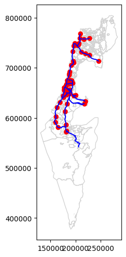
Here is the plot of the towns, stations, and rail layers, together (see Plotting more than one layer):
base = towns.plot(color='white', edgecolor='lightgrey')
stations.plot(ax=base, color='red')
rail.plot(ax=base, color='blue');
CRS and reprojection#
What is a CRS?#
A Coordinate Reference System (CRS) defines the association between coordinates (which are ultimately just numbers) and specific locations on the surface of the earth. CRS can be divided into two groups:
Geographic CRS, where units are degrees (e.g., WGS84)
Projected CRS, where units are “real” distance units, typically meters (e.g., ITM, UTM)
There are several methods and formats to describe and specify a CRS. The shortest and simplest method is to use an EPSG code, which all standard CRS have. For example, Table 23 specifies the EPSG codes of CRS we encounter in this book.
Name |
Type |
Units |
EPSG code |
|---|---|---|---|
WGS84 |
Geographic |
Decimal degrees (\(^\circ\)) |
|
ITM |
Projected |
Meters (\(m\)) |
|
UTM Zone 36N |
Projected |
Meters (\(m\)) |
|
Geographic CRS refer to the entire surface of the Earth, while projected CRS commonly refer to smaller areas. A fundamental difference between geographical and projected CRS is in their units. Geographic CRS refer to location on a sphere, using degree units, while projected CRS refer to locations on an approximated planar surface. One important implication of the unit difference is that planar gemetric calculations (such as distance and area) make sense in projected CRS, but not in geographic CRS.
Note
There are several formats, or standards, to specify a CRS, in Python and elsewhere. The most common ones are:
EPSG code—e.g.,
4326PROJ string—e.g.,
'+proj=longlat +datum=WGS84 +no_defs'WKT string—e.g.,
'GEOGCS["WGS 84",DATUM["WGS_1984",...[etc.]'
In this book, we exclusively use EPSG codes to define projections, for their simplicity.
Examining with .crs#
As mentioned previously (see GeoDataFrame structure), the CRS definition of a GeoSeries (or GeoDataFrame) is accessible through the .crs property. For example, here is the CRS definition of the rail layer:
rail.crs
<Projected CRS: EPSG:2039>
Name: Israel 1993 / Israeli TM Grid
Axis Info [cartesian]:
- E[east]: Easting (metre)
- N[north]: Northing (metre)
Area of Use:
- name: Israel - onshore; Palestine Territory - onshore.
- bounds: (34.17, 29.45, 35.69, 33.28)
Coordinate Operation:
- name: Israeli TM
- method: Transverse Mercator
Datum: Israel 1993
- Ellipsoid: GRS 1980
- Prime Meridian: Greenwich
The rail layer is in the ITM system. The EPSG code of this CRS is 2039. Exploring the printout can also reveal that the CRS units are meters, and that the geographical area where the CRS is supposed to be used is Israel.
Modifying with .set_crs#
To modify the CRS definition of a given layer, we can use the .set_crs method. In case the layer already has a CRS definition, we must use the allow_override=True option. Otherwise, we get an error. The allow_override argument is a safeguard against replacing the CRS definition of a layer when it already has one, which only makes sense if the existing CRS definition is wrong and we need to “fix” it (see below).
For example, the following expression replaces the CRS definition of rail (which is ITM, 2039) with another CRS (WGS84, 4326):
rail = rail.set_crs(4326, allow_override=True)
We can examine the .crs property, to see that the CRS definition has indeed changed:
rail.crs
<Geographic 2D CRS: EPSG:4326>
Name: WGS 84
Axis Info [ellipsoidal]:
- Lat[north]: Geodetic latitude (degree)
- Lon[east]: Geodetic longitude (degree)
Area of Use:
- name: World.
- bounds: (-180.0, -90.0, 180.0, 90.0)
Datum: World Geodetic System 1984 ensemble
- Ellipsoid: WGS 84
- Prime Meridian: Greenwich
It is important to note that replacing the CRS definition has no effect on the coordinates. For example, the coordinates of rail are still in ITM units, rather than decimal degrees:
print(rail.geometry.iloc[11])
LINESTRING (188700.04908514675 648249.5428679045, 188521.65428514872 648456.553667903)
This means that the layer is now incorrect (!), since the coordinates do not match the CRS definition. Replacing the CRS definition should only be done when:
The layer has no CRS definition, e.g., it was accidentally lost, and we need to restore it
The existing CRS definition is incorrect, and we need to replace it with the correct one
Let’s modify the CRS definition back to the original, to “fix” the layer we have just broken:
rail = rail.set_crs(2039, allow_override=True)
Note
To remove the CRS definition of a given layer altogether, you can assign None to the .crs property, as in rail.crs=None.
Reprojecting with .to_crs#
Reprojecting a vector layer involves not just replacing the CRS definition (see Modifying with .set_crs), but also re-calculating all of the layer coordinates, so that they are in agreement with the new CRS.
To reproject a GeoSeries or GeoDataFrame, we use the .to_crs method. For example, here is how we can transform the rail layer to WGS84:
rail = rail.to_crs(4326)
Comparing the updated .crs property of rail with the original one (see above), we can see that the CRS definition indeed changed:
rail.crs
<Geographic 2D CRS: EPSG:4326>
Name: WGS 84
Axis Info [ellipsoidal]:
- Lat[north]: Geodetic latitude (degree)
- Lon[east]: Geodetic longitude (degree)
Area of Use:
- name: World.
- bounds: (-180.0, -90.0, 180.0, 90.0)
Datum: World Geodetic System 1984 ensemble
- Ellipsoid: WGS 84
- Prime Meridian: Greenwich
Importantly, the coordinates also changed, which can be demonstrated by printing the WKT representation of any given geometry from the layer (compare with the above printout):
print(rail.geometry.iloc[11])
LINESTRING (34.87921676021756 31.926817568737928, 34.87732378978819 31.928679560071494)
Thus the information in the rail layer is still “correct”, as the coordinates match the CRS. It is just in a different CRS.
Finally, we can see that the axis text labels when plotting the layer have changed, now reflecting decimal degree values of the WGS84 CRS:
rail.plot();
Let us reproject rail back to the original CRS (i.e., ITM) before we proceed:
rail = rail.to_crs(epsg=2039)
Note
More information on specifying projections, and reprojecting layers, can be found in the Projections article.
Numeric calculations#
Overview#
In this section, we cover commonly-used geometric calculations that result in numeric values, using geopandas. As we will see, the first three operations are very similar to their shapely counterparts (Table 24). The difference is that the calculation is applied on multiple geometries, rather than just one.
Method |
|
|
|---|---|---|
|
see Length (shapely) |
|
|
see Area (shapely) |
see Area (geopandas) |
|
The fourth operation, detecting nearest neighbors, which we cover last (see Nearest neighbors), is a little more complex and not really analogous to any shapely-based workflow.
Length (geopandas)#
The .length property returns a Series with line lengths per geometry in a GeoSeries or GeoDataFrame. For example, rail.length returns a Series of railway segment lengths:
rail.length
0      12379.715331
1       2274.111799
3       2793.337699
4       1960.170882
5       1195.701220
           ...
210     5975.045997
211     1913.384027
214     1603.616014
215      166.180958
216     1284.983680
Length: 161, dtype: float64
Keep in mind that all numeric calculations, such as length, area (see Area (geopandas)), and distance (see Distance (geopandas)), are returned in the coordinate units, that is, in CRS units. In our case, the CRS is ITM, where the units are meters (\(m\)) (Table 23). The following expression transforms the values from \(m\) to \(km\):
rail.length / 1000
0      12.379715
1       2.274112
3       2.793338
4       1.960171
5       1.195701
         ...
210     5.975046
211     1.913384
214     1.603616
215     0.166181
216     1.284984
Length: 161, dtype: float64
This Series can be assigned to into a new column, such as a column named 'length_km', as follows:
rail['length_km'] = rail.length / 1000
rail
| SEGMENT | geometry | length_km | |
|---|---|---|---|
| 0 | כפר יהושע - נשר_1 | LINESTRING (205530.083 741562.9... | 12.379715 |
| 1 | באר יעקב-ראשונים_2 | LINESTRING (181507.598 650706.1... | 2.274112 |
| 3 | לב המפרץ מזרח - נשר_4 | LINESTRING (203482.789 744181.5... | 2.793338 |
| 4 | קרית גת - להבים_5 | LINESTRING (178574.101 609392.9... | 1.960171 |
| 5 | רמלה - רמלה מזרח_6 | LINESTRING (189266.58 647211.50... | 1.195701 |
| ... | ... | ... | ... |
| 210 | ויתקין - חדרה_215 | LINESTRING (190758.23 704950.04... | 5.975046 |
| 211 | בית יהושע - נתניה ספיר_216 | LINESTRING (187526.597 687360.3... | 1.913384 |
| 214 | השמונה - בית המכס_220 | LINESTRING (200874.999 746209.3... | 1.603616 |
| 215 | לב המפרץ - בית המכס_221 | LINESTRING (203769.786 744358.6... | 0.166181 |
| 216 | 224_לוד מרכז - נתבג | LINESTRING (190553.481 654170.3... | 1.284984 |
161 rows × 3 columns
All geometric operations in geopandas assume planar geometry, returning the result in the CRS units. This means that layers in a geographic CRS (such as WGS84) need to be transformed to a projected CRS (see What is a CRS?) before any geometric calculation. Otherwise, numeric measurements, such as length, area, and distance, are going to be returned in decimal degree units, which usually does not make sense, as the relation between degrees and geographic distance is not a fixed one.
Exercise 09-a
Reproject the
raillayer to geographic coordinates (4326), then calculate railway lengths once again. You should see the (meaningless) results in decimal degrees.
Area (geopandas)#
The .area property returns a Series with the area per geometry in a GeoSeries or GeoDataFrame. For example, towns.area returns the area sizes of each polygon in the towns layer, again in CRS units (\(m^2\)):
towns.area
0      2.721176e+07
1      7.708050e+04
2      1.043253e+06
3      4.769053e+04
4      2.144091e+04
           ...
406    2.001376e+05
407    2.246316e+05
408    1.141930e+06
409    4.076764e+04
410    3.961142e+06
Length: 411, dtype: float64
If necessary, this series can be assigned to a new column. For example, the following expression divides the area values by \(1000^2\), i.e., 1000**2 to convert from \(m^2\) to \(km^2\), then assigns the results to a new column named 'area_km2':
towns['area_km2'] = towns.area / 1000**2
towns
| Muni_Heb | Machoz | Shape_Area | geometry | area_km2 | |
|---|---|---|---|---|---|
| 0 | שפיר | דרום | 2.721176e+07 | POLYGON Z ((177281.694 610056.5... | 27.211760 |
| 1 | דימונה | דרום | 7.708050e+04 | POLYGON Z ((205753.745 560693.6... | 0.077080 |
| 2 | דימונה | דרום | 1.043253e+06 | POLYGON Z ((207740.171 563476.5... | 1.043253 |
| 3 | זבולון | חיפה | 4.769053e+04 | POLYGON Z ((209445.229 740507.2... | 0.047691 |
| 4 | מגידו | צפון | 2.144091e+04 | POLYGON Z ((206769.626 727131.7... | 0.021441 |
| ... | ... | ... | ... | ... | ... |
| 406 | ללא שיפוט - אזור מעיליא | צפון | 2.001376e+05 | POLYGON Z ((225369.655 770523.6... | 0.200138 |
| 407 | זבולון | חיפה | 2.246316e+05 | POLYGON Z ((207596.214 746263.0... | 0.224632 |
| 408 | זבולון | חיפה | 1.141930e+06 | POLYGON Z ((208622.688 746540.1... | 1.141930 |
| 409 | רמת השרון | תל אביב | 4.076764e+04 | POLYGON Z ((183576.756 673627.0... | 0.040768 |
| 410 | צור הדסה | ירושלים | 3.961142e+06 | POLYGON Z ((209871.005 625364.9... | 3.961142 |
411 rows × 5 columns
Exercise 09-b
Find out the names of the largest and the smallest municipal area polygon, in terms of area size, based on the
townslayer. (answer:'ללא שיפוט - אזור נחל ארבל'and'רמת נגב')
Exercise 09-c
Check the association between the
'area_km2'column we calculated, and the'Shape_Area'column which is stored in the Shapefile, using a scatterplot (see Scatterplots (pandas)) (Fig. 56).
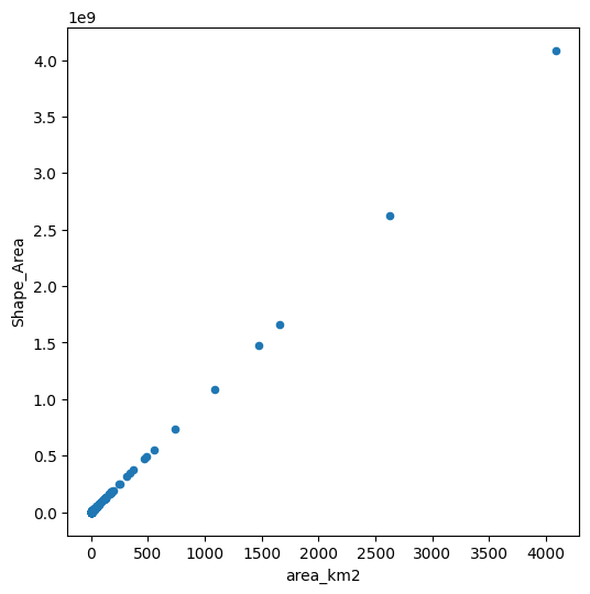
Fig. 56 Solution of exercise-09-c: Association between the (calculated) 'area_km2' column and the (original) 'Shape_Area' column#
Distance (geopandas)#
The .distance method can be used to calculate distances. Each distance is calculated exactly the same way as in shapely, i.e., minimal distance between the geometries assuming planar coordinates. However, since we are dealing with multiple inputs, the geopandas mode of operation is different. Specifically, the geopandas operation of .distance (and other pairwise methods, see below) can work in two “modes”:
Many-to-One— when the “second” argument is a
shapelygeometry (Fig. 57, left)Pairwise—when the “second” argument is a
GeoSeries(Fig. 57, right)

Fig. 57 geopandas modes of operation for methods accepting pairs of inputs, such as .distance: many-to-one (left) and pairwise (right) (Source: https://geopandas.org/en/stable/docs/reference/api/geopandas.GeoSeries.distance.html)#
The following example demonstrates the many-to-one option. Here, we are calculating the distances between:
stations—all railway stations, andrail.geometry.iloc[0]—the first railway segment.
The result is a Series of distances, in \(m\):
stations.distance(rail.geometry.iloc[0])
0      84284.975205
1      50424.920267
2      74235.170679
3     138847.580690
4      86603.473121
          ...
58      8595.362486
59    160138.041969
60      9758.724335
61     84904.898970
62     26515.877484
Length: 63, dtype: float64
What if we need to calculate the complete matrix of pairwise distances, between each station and each railway segment? This can be done using .apply (see apply and custom functions). The following expression, in plain language, means that we take each row (axis=1) in stations as x, then calculate the Series of distances from all railway segments to the geometry of that row (rail.distance(x.geometry)).
The result is a DataFrame representing a distance matrix, where:
Rows represent railway stations
Columns represent railway segments
Cell values are distances, in meters
d = stations.apply(lambda x: rail.distance(x.geometry), axis=1)
d
| 0 | 1 | 3 | 4 | 5 | ... | 210 | 211 | 214 | 215 | 216 | |
|---|---|---|---|---|---|---|---|---|---|---|---|
| 0 | 84284.975205 | 6120.325293 | 91266.392666 | 43769.104489 | 13360.106887 | ... | 46002.039665 | 31998.139305 | 94172.402848 | 93091.940077 | 13376.996382 |
| 1 | 50424.920267 | 37379.975682 | 57120.870160 | 76795.773036 | 39353.653794 | ... | 11924.365438 | 236.552504 | 60107.821537 | 58958.887738 | 33548.162167 |
| 2 | 74235.170679 | 13859.386195 | 81199.631964 | 53259.279461 | 18180.867522 | ... | 35958.589113 | 21932.455984 | 84145.901064 | 83037.130172 | 14356.406044 |
| 3 | 138847.580690 | 51367.336965 | 146064.901194 | 19030.199927 | 52794.173376 | ... | 100790.724935 | 86796.547920 | 148925.381315 | 147885.212962 | 58403.590869 |
| 4 | 86603.473121 | 5697.560021 | 94960.212976 | 38438.916853 | 289.422152 | ... | 50857.456340 | 37074.116175 | 98521.682411 | 97044.665341 | 4964.211497 |
| ... | ... | ... | ... | ... | ... | ... | ... | ... | ... | ... | ... |
| 58 | 8595.362486 | 86339.689331 | 20244.761995 | 123902.486603 | 85772.327241 | ... | 37220.552915 | 52057.048736 | 26186.457201 | 22822.683088 | 79583.761529 |
| 59 | 160138.041969 | 74611.504901 | 169029.718846 | 34992.788653 | 73042.322269 | ... | 125012.376699 | 111083.909066 | 172714.053593 | 171172.498821 | 78870.029306 |
| 60 | 9758.724335 | 99222.671750 | 6473.850217 | 138574.693149 | 100683.138956 | ... | 44196.792329 | 62080.870950 | 1709.845960 | 6471.883040 | 94617.022408 |
| 61 | 84904.898970 | 5579.557103 | 93200.557041 | 40156.246177 | 2075.672842 | ... | 49040.957113 | 35245.583872 | 96738.721423 | 95275.546196 | 3553.733949 |
| 62 | 26515.877484 | 120379.789258 | 24360.621700 | 159481.427917 | 121328.202345 | ... | 65575.558369 | 83375.846025 | 22375.584322 | 24118.556926 | 115179.615344 |
63 rows × 161 columns
Note that the first column in the above result is identical to the Series we got in the previous expression.
The distance matrix can be refined to calculate more specific properties related to distance that we are interested in. For example, to get the minimum distance to any of the railway segments (rather than all distances), we can apply the .min() method on each row, as follows. The result is a Series of minimal distances per station:
nearest_seg_dist = d.min(axis=1)
nearest_seg_dist
0      13.440327
1       4.932094
2      16.180832
3      64.381044
4       2.941401
         ...
58     56.102377
59      7.540327
60     44.130049
61     22.556829
62    115.502833
Length: 63, dtype: float64
We can assign it to a new column named 'nearest_seg_dist' (“distance to nearest segment”) in stations, as follows:
stations['nearest_seg_dist'] = nearest_seg_dist
stations
| STAT_NAMEH | OFF_7_DAY | geometry | nearest_seg_dist | |
|---|---|---|---|---|
| 0 | ראשון לציון משה דיין | 72.0 | POINT (177206.094 655059.936) | 13.440327 |
| 1 | קרית ספיר נתניה | 119.0 | POINT (187592.123 687587.598) | 4.932094 |
| 2 | ת"א השלום | 1642.0 | POINT (180621.94 664537.21) | 16.180832 |
| 3 | שדרות | 26.0 | POINT (160722.849 602798.889) | 64.381044 |
| 4 | רמלה | 47.0 | POINT (188508.91 648466.87) | 2.941401 |
| ... | ... | ... | ... | ... |
| 58 | מגדל העמק כפר ברוך | 5.0 | POINT (219851.931 728164.825) | 56.102377 |
| 59 | באר שבע אוניברסיטה | 130.0 | POINT (181813.614 574550.411) | 7.540327 |
| 60 | חיפה בת גלים | 311.0 | POINT (198610.01 748443.79) | 44.130049 |
| 61 | לוד | 238.0 | POINT (188315.977 650289.373) | 22.556829 |
| 62 | נהריה | 64.0 | POINT (209570.59 767769.22) | 115.502833 |
63 rows × 4 columns
Nearest neighbors#
Here is another technique to extract information from the distance matrix, expanding the above expression of distance to nearest neighbor. This time, we calculate the name ('SEGMENT' column) of the nearest railway segment for each station. We are using the .idxmin method (see Table 14), instead of .min, to get the index of the nearest segment (instead of the distance to it):
ids = d.idxmin(axis=1)
ids
0      22
1     100
2      57
3     131
4      87
     ...
58    152
59    205
60    153
61     77
62     12
Length: 63, dtype: int64
The index can be used to subset segment names (rail['SEGMENT']). The result is a series of the nearest segment names:
nearest_seg_name = rail['SEGMENT'].loc[ids]
nearest_seg_name
22              משה דיין-קוממיות_23
100    נתניה מכללה - נתניה ספיר_101
57           סבידור מרכז - השלום_58
131              שדרות-יד מרדכי_134
87                    לוד - רמלה_88
                   ...
152            עפולה - כפר ברוך_155
205    באר שבע צפון - באר שבע אוניב
153          חוף כרמל - בת גלים_156
77                    לוד - רמלה_78
12                   נהריה - עכו_13
Name: SEGMENT, Length: 63, dtype: object
Let’s attach the result to another column in the stations table, named nearest_seg_name (“nearest segment name”). We need to reset the indices to make sure the column is attached by position:
nearest_seg_name = nearest_seg_name.reset_index(drop=True)
nearest_seg_name
0              משה דיין-קוממיות_23
1     נתניה מכללה - נתניה ספיר_101
2           סבידור מרכז - השלום_58
3               שדרות-יד מרדכי_134
4                    לוד - רמלה_88
                  ...
58            עפולה - כפר ברוך_155
59    באר שבע צפון - באר שבע אוניב
60          חוף כרמל - בת גלים_156
61                   לוד - רמלה_78
62                  נהריה - עכו_13
Name: SEGMENT, Length: 63, dtype: object
stations['nearest_seg_name'] = nearest_seg_name
stations
| STAT_NAMEH | OFF_7_DAY | geometry | nearest_seg_dist | nearest_seg_name | |
|---|---|---|---|---|---|
| 0 | ראשון לציון משה דיין | 72.0 | POINT (177206.094 655059.936) | 13.440327 | משה דיין-קוממיות_23 |
| 1 | קרית ספיר נתניה | 119.0 | POINT (187592.123 687587.598) | 4.932094 | נתניה מכללה - נתניה ספיר_101 |
| 2 | ת"א השלום | 1642.0 | POINT (180621.94 664537.21) | 16.180832 | סבידור מרכז - השלום_58 |
| 3 | שדרות | 26.0 | POINT (160722.849 602798.889) | 64.381044 | שדרות-יד מרדכי_134 |
| 4 | רמלה | 47.0 | POINT (188508.91 648466.87) | 2.941401 | לוד - רמלה_88 |
| ... | ... | ... | ... | ... | ... |
| 58 | מגדל העמק כפר ברוך | 5.0 | POINT (219851.931 728164.825) | 56.102377 | עפולה - כפר ברוך_155 |
| 59 | באר שבע אוניברסיטה | 130.0 | POINT (181813.614 574550.411) | 7.540327 | באר שבע צפון - באר שבע אוניב |
| 60 | חיפה בת גלים | 311.0 | POINT (198610.01 748443.79) | 44.130049 | חוף כרמל - בת גלים_156 |
| 61 | לוד | 238.0 | POINT (188315.977 650289.373) | 22.556829 | לוד - רמלה_78 |
| 62 | נהריה | 64.0 | POINT (209570.59 767769.22) | 115.502833 | נהריה - עכו_13 |
63 rows × 5 columns
The last example can be considered as a “manually” constructed nearest-neighbor spatial join, since we actually joined an attribute ('SEGMENT') value from one layer (rail) to another layer (stations), based on minimum distance. Towards the end of this chapter we will introduce the the gpd.sjoin_nearest function which can do nearest-neighbor spatial join automatically (see Nearest neighbor join).
New geometries 1 (geopandas)#
Overview#
In this section and the next one, we learn about functions that calculate new geometries. We are already familiar with this type of operations for individual geometry objects, using shapely (see New geometries 1 (shapely) and New geometries 2 (shapely)). Now, we learn about the same type of operations for vector layers, which include more than one geometry. Similarly to our treatment of shapely methods, we split the discussion into two parts: operations on single geometries (this section), and operations on pairs of geometries (New geometries 2 (geopandas)).
The single-geometry methods are similar to the shapely methods (Table 25), only that they accept a GeoSeries (or GeoDataFrame) and return a new GeoSeries with the results. In fact, the geopandas methods are simply “wrappers” of the respective shapely methods. We will demonstrate just the two most commonly used methods, .centroid (Centroids (geopandas)) and .buffer (Buffers (geopandas)). For example, when applying .centroid on a vector layer or geometry column, we get a new geometry column, with the same number of geometries as the original, where each geometry is the centroid of the respective original geometry.
Property or Method |
Meaning |
|---|---|
Convex Hull |
|
Envelope |
|
Minimum rotated rectangle |
|
Simplified geometry |
Centroids (geopandas)#
The .centroid method, applied on a GeoSeries or GeoDataFrame, returns a new GeoSeries with the centroids. For example, here is how we can create a GeoSeries of town polygon centroids:
ctr = towns.centroid
ctr
0      POINT (177487.729 608814.771)
1      POINT (205649.879 560604.535)
2      POINT (207998.865 562886.601)
3      POINT (209338.568 740382.523)
4      POINT (206932.541 727058.938)
                   ...
406    POINT (225182.898 770809.745)
407     POINT (208021.906 746132.09)
408     POINT (208513.59 747266.263)
409    POINT (183415.358 673541.053)
410    POINT (209371.055 625163.901)
Length: 411, dtype: geometry
And here is a plot of the result:
ctr.plot(markersize=15, edgecolor='black');
Buffers (geopandas)#
The .buffer method buffers each geometry in a given GeoDataFrame or GeoSeries to the specified distance. It returns a GeoSeries with the resulting polygons. For example, here we create buffers of 5,000 \(m\) (i.e., 5 \(km\)) around each railway station:
stations_buffer = stations.buffer(5000)
stations_buffer
0     POLYGON ((182206.094 655059.936...
1     POLYGON ((192592.123 687587.598...
2     POLYGON ((185621.94 664537.21, ...
3     POLYGON ((165722.849 602798.889...
4     POLYGON ((193508.91 648466.87, ...
                     ...
58    POLYGON ((224851.931 728164.825...
59    POLYGON ((186813.614 574550.411...
60    POLYGON ((203610.01 748443.79, ...
61    POLYGON ((193315.977 650289.373...
62    POLYGON ((214570.59 767769.22, ...
Length: 63, dtype: geometry
Here is a plot of the result:
stations_buffer.plot(color='none');
Exercise 09-d
As shown above, centroids and buffers are returned as a
GeoSeriesSuppose that, instead, you need a
GeoDataFramewith the original attributes of the source layer (e.g., the railway station properties) and the centroid, or buffer, geometries. How can we create suchGeoDataFrames?
New geometries 2 (geopandas)#
Pairwise methods#
geopandas defines analogous pairwise methods (Table 26), with the same functionality as those we are familiar from shapely (Table 22).
Method |
Meaning |
|---|---|
Intersection |
|
Union |
|
Difference |
|
Symmetric difference |
The methods listed in Table 26 can also be used in the two modes mentioned for .distance (Distance (geopandas)), namely many-to-one or pairwise (Fig. 57). In the following example we demonstrate the first mode (many-to-one), which is both simpler and more useful. For the first (“many”) input we’ll take towns, while for the second (“one”) geometry, we’ll take a particular railway segment, part of the line that goes from Tel-Aviv to Jerusalem:
seg = rail[rail['SEGMENT'] == 'נתבג - יצחק נבון_198']
seg
| SEGMENT | geometry | length_km | |
|---|---|---|---|
| 194 | נתבג - יצחק נבון_198 | LINESTRING (194999.696 643851.4... | 27.985833 |
Given towns and seg, we will calculate pairwise intersections, that is, the segment portions that go through each town.
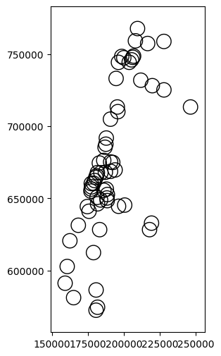
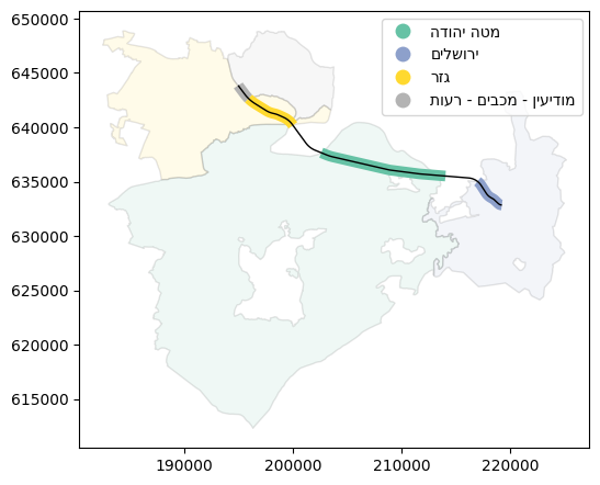
An interactive map of the inputs, seg and the towns features it intersects with, is shown below. Note that we are using .intersects to subset the towns layer, which will be explained later (Boolean methods (geopandas)). Also note the technique being used to show two different layers in the same .explore plot (similar to what we learned about .plot, see Plotting more than one layer).
m = towns[towns.intersects(seg.union_all())].explore()
seg.explore(m = m, color='red', style_kwds={'weight':8, 'opacity':0.8})
Here is how we can use the .intersection method to find the intersections of all town polygons (many) with the railway segment seg (one). We’ll call the result seg1:
seg1 = towns.intersection(seg.geometry.iloc[0])
seg1
0      LINESTRING Z EMPTY
1      LINESTRING Z EMPTY
2      LINESTRING Z EMPTY
3      LINESTRING Z EMPTY
4      LINESTRING Z EMPTY
              ...
406    LINESTRING Z EMPTY
407    LINESTRING Z EMPTY
408    LINESTRING Z EMPTY
409    LINESTRING Z EMPTY
410    LINESTRING Z EMPTY
Length: 411, dtype: geometry
seg1 is a GeoSeries of the same lenght of towns, with the intersections between each town and the segment seg. Naturally, most of the resulting geometries are empty, since there are no intersections between most towns and the one particular railway segment. We can filter out empty geometries using the .is_empty property:
seg1 = seg1[~seg1.is_empty]
seg1
161    LINESTRING Z (194999.696 643851...
268    LINESTRING Z (195949.355 642639...
300    LINESTRING Z (217013.82 635020....
328    LINESTRING Z (202640.669 637654...
dtype: geometry
Also, let’s switch to a GeoDataFrame representation:
seg1 = gpd.GeoDataFrame(geometry=seg1)
seg1
| geometry | |
|---|---|
| 161 | LINESTRING Z (194999.696 643851... |
| 268 | LINESTRING Z (195949.355 642639... |
| 300 | LINESTRING Z (217013.82 635020.... |
| 328 | LINESTRING Z (202640.669 637654... |
Here is the result:
seg1.plot();
Typically we want to know the details of each segment, such as the attributes of the town it goes through. Using pd.concat (see Concatenation), we can combine seg1 with matching attributes from towns (aligned by index):
seg1 = pd.concat([seg1, towns[['Muni_Heb']]], axis=1, join='inner')
seg1
| geometry | Muni_Heb | |
|---|---|---|
| 161 | LINESTRING Z (194999.696 643851... | מודיעין - מכבים - רעות |
| 268 | LINESTRING Z (195949.355 642639... | גזר |
| 300 | LINESTRING Z (217013.82 635020.... | ירושלים |
| 328 | LINESTRING Z (202640.669 637654... | מטה יהודה |
Now we have the geometry of each seg part which goes through every particular town, as well as the properties of that town.
Note
Alternatively, we could use the .join method (of pandas) to combine two tables by index, which has shorter and cleaner syntax for this case:
seg1.join(towns[['Muni_Heb']])
To plot the result with a legend, we have to resort to a trick to reverse the town name strings. Otherwise, the Hebrew text is shown in reverse order:
towns1 = towns[towns.intersects(seg1.union_all())]
towns1.loc[:, 'Muni_Heb'] = towns1['Muni_Heb'].apply(lambda x: x[::-1])
seg1.loc[:, 'Muni_Heb'] = seg1['Muni_Heb'].apply(lambda x: x[::-1])
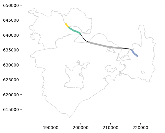
Here is a plot of:
The town polygons
towns(in color, according toMuni_Heb)The railway segment
seg(in black)The intersection result
seg1(in color, according toMuni_Heb)
base = towns1.plot(column='Muni_Heb', cmap='Set2', edgecolor='black', alpha=0.1)
seg1.plot(ax=base, column='Muni_Heb', cmap='Set2', linewidth=7, legend=True)
seg.plot(ax=base, color='black', linewidth=1);
Set-operations (.overlay)#
In addition to the standard methods, such as .intersection (Pairwise methods), geopandas defines the .overlay method. Using .overlay, we can “split” one layer with another, while keeping the original attributes of both inputs, for each part. The how argument determines which of the parts are returned. For example:
how='intersection'—returns only the shared partshow='union'—returns all parts
The complete list of .overlay(how=...) options is given in Table 27.
Method |
Meaning |
|---|---|
|
Shared parts only |
|
All parts |
|
Parts of the first geometry only (without shared) |
|
Parts of the first or second geometry (without shared) |
|
Parts of the first geometry or shared |
This will be made clear in the following example. The following .overlay expression calculates the pairwise intersections between railway segments (rail) and towns (towns), creating a new layer of pairwise intersections rail_towns:
rail_towns = rail.overlay(towns[['Muni_Heb', 'geometry']])
rail_towns
| SEGMENT | length_km | Muni_Heb | geometry | |
|---|---|---|---|---|
| 0 | כפר יהושע - נשר_1 | 12.379715 | ללא שיפוט - אזור הר הכרמל | LINESTRING Z (209316.903 736321... |
| 1 | כפר יהושע - נשר_1 | 12.379715 | נשר | LINESTRING Z (205530.083 741562... |
| 2 | כפר יהושע - נשר_1 | 12.379715 | קרית טבעון | LINESTRING Z (210111.094 732877... |
| 3 | כפר יהושע - נשר_1 | 12.379715 | זבולון | LINESTRING Z (206157.238 740691... |
| 4 | כפר יהושע - נשר_1 | 12.379715 | עמק יזרעאל | LINESTRING Z (210658.396 732427... |
| ... | ... | ... | ... | ... |
| 278 | בית יהושע - נתניה ספיר_216 | 1.913384 | נתניה | LINESTRING Z (187526.597 687360... |
| 279 | בית יהושע - נתניה ספיר_216 | 1.913384 | חוף השרון | LINESTRING Z (187356.05 686718.... |
| 280 | השמונה - בית המכס_220 | 1.603616 | חיפה | LINESTRING Z (200874.999 746209... |
| 281 | לב המפרץ - בית המכס_221 | 0.166181 | חיפה | LINESTRING Z (203769.786 744358... |
| 282 | 224_לוד מרכז - נתבג | 1.284984 | שדות דן | LINESTRING Z (190553.481 654170... |
283 rows × 4 columns
To understand what has happened, consider the specific segment in the rail layer from the last example (Pairwise methods):
rail[rail['SEGMENT'] == 'נתבג - יצחק נבון_198']
| SEGMENT | geometry | length_km | |
|---|---|---|---|
| 194 | נתבג - יצחק נבון_198 | LINESTRING (194999.696 643851.4... | 27.985833 |
In the result of the overlay operation rail_towns, this particular segment was split into four parts, as it crosses four different polygons from the towns layer. We can see, in the result, the names of those towns features:
seg = rail_towns[rail_towns['SEGMENT'] == 'נתבג - יצחק נבון_198']
seg
| SEGMENT | length_km | Muni_Heb | geometry | |
|---|---|---|---|---|
| 257 | נתבג - יצחק נבון_198 | 27.985833 | מודיעין - מכבים - רעות | LINESTRING Z (194999.696 643851... |
| 258 | נתבג - יצחק נבון_198 | 27.985833 | גזר | LINESTRING Z (195949.355 642639... |
| 259 | נתבג - יצחק נבון_198 | 27.985833 | ירושלים | LINESTRING Z (217013.82 635020.... |
| 260 | נתבג - יצחק נבון_198 | 27.985833 | מטה יהודה | LINESTRING Z (202640.669 637654... |
as demonstrated in the following plot:
base = towns[towns.intersects(seg.union_all())].plot(color='none', edgecolor='lightgrey')
seg.plot(ax=base, column='Muni_Heb', cmap='Set2', linewidth=4, missing_kwds={'color':'black', 'linewidth':1});
Thus, .overlay with how='intersection' can be thought of as an expanded version of .intersection (Pairwise methods), where we calculate intersection in a “many-to-many” mode (between all towns and all railway segments), and also get the respective attributes without having to manually join them.
You may notice that only overlapping parts of the two layers were returned, as a result of (the default) how='intersection' setting of .overlay. To get all parts, we could use how='union':
rail_towns = rail.overlay(towns[['Muni_Heb', 'geometry']], how='union')
rail_towns
/home/michael/Sync/venv/m/lib/python3.12/site-packages/geopandas/geodataframe.py:2675: UserWarning: `keep_geom_type=True` in overlay resulted in 411 dropped geometries of different geometry types than df1 has. Set `keep_geom_type=False` to retain all geometries
  return geopandas.overlay(
| SEGMENT | length_km | Muni_Heb | geometry | |
|---|---|---|---|---|
| 0 | כפר יהושע - נשר_1 | 12.379715 | ללא שיפוט - אזור הר הכרמל | LINESTRING Z (209316.903 736321... |
| 1 | כפר יהושע - נשר_1 | 12.379715 | נשר | LINESTRING Z (205530.083 741562... |
| 2 | כפר יהושע - נשר_1 | 12.379715 | קרית טבעון | LINESTRING Z (210111.094 732877... |
| 3 | כפר יהושע - נשר_1 | 12.379715 | זבולון | LINESTRING Z (206157.238 740691... |
| 4 | כפר יהושע - נשר_1 | 12.379715 | עמק יזרעאל | LINESTRING Z (210658.396 732427... |
| ... | ... | ... | ... | ... |
| 302 | בני ברק - קרית אריה_191 | 3.135967 | NaN | LINESTRING Z (185847.279 667798... |
| 303 | נתבג - יצחק נבון_198 | 27.985833 | NaN | MULTILINESTRING Z ((200031.323 ... |
| 304 | קרית מוצקין - סביוני ים_212 | 3.555612 | NaN | LINESTRING Z (207382.568 749536... |
| 305 | בית יהושע - נתניה ספיר_216 | 1.913384 | NaN | LINESTRING Z (187356.05 686718.... |
| 306 | NaN | NaN | מגדל | LINESTRING Z (246764.475 748264... |
307 rows × 4 columns
Note
The above .overlay(..., how='union') expression returns all parts of both input layers but only if they are of the same type (lines!) as the first input layer rail. This is the default keep_geom_type=True behavior. In this case, it’s exactly what we want; otherwise we would get all parts of the town polygons as well.
Now, our particular rail segment (as well as any other segment) was split to parts per town, but also has a separate part for the those sections that do not overlap with any towns, if any (with Muni_Heb set to np.nan):
seg = rail_towns[rail_towns['SEGMENT'] == 'נתבג - יצחק נבון_198']
seg
| SEGMENT | length_km | Muni_Heb | geometry | |
|---|---|---|---|---|
| 257 | נתבג - יצחק נבון_198 | 27.985833 | מודיעין - מכבים - רעות | LINESTRING Z (194999.696 643851... |
| 258 | נתבג - יצחק נבון_198 | 27.985833 | גזר | LINESTRING Z (195949.355 642639... |
| 259 | נתבג - יצחק נבון_198 | 27.985833 | ירושלים | LINESTRING Z (217013.82 635020.... |
| 260 | נתבג - יצחק נבון_198 | 27.985833 | מטה יהודה | LINESTRING Z (202640.669 637654... |
| 303 | נתבג - יצחק נבון_198 | 27.985833 | NaN | MULTILINESTRING Z ((200031.323 ... |
The plot demonstrates the new result (we use missing_kwds to make sure features with “No Data” for Muni_Heb are also plotted):
base = towns[towns.intersects(seg.union_all())].plot(color='none', edgecolor='lightgrey')
seg.plot(ax=base, column='Muni_Heb', cmap='Set2', linewidth=4, missing_kwds={'color':'black', 'linewidth':1});
Note that the length_km attribute was “inherited” from the original rail layer, and it no longer represents the length of the sub-segments resulting from the overlay operation:
seg
| SEGMENT | length_km | Muni_Heb | geometry | |
|---|---|---|---|---|
| 257 | נתבג - יצחק נבון_198 | 27.985833 | מודיעין - מכבים - רעות | LINESTRING Z (194999.696 643851... |
| 258 | נתבג - יצחק נבון_198 | 27.985833 | גזר | LINESTRING Z (195949.355 642639... |
| 259 | נתבג - יצחק נבון_198 | 27.985833 | ירושלים | LINESTRING Z (217013.82 635020.... |
| 260 | נתבג - יצחק נבון_198 | 27.985833 | מטה יהודה | LINESTRING Z (202640.669 637654... |
| 303 | נתבג - יצחק נבון_198 | 27.985833 | NaN | MULTILINESTRING Z ((200031.323 ... |
If necessary, we can “update” the length attribute by recalculating geometry lengths:
rail_towns['length_km'] = rail_towns.length / 1000
seg = rail_towns[rail_towns['SEGMENT'] == 'נתבג - יצחק נבון_198']
seg
| SEGMENT | length_km | Muni_Heb | geometry | |
|---|---|---|---|---|
| 257 | נתבג - יצחק נבון_198 | 1.541502 | מודיעין - מכבים - רעות | LINESTRING Z (194999.696 643851... |
| 258 | נתבג - יצחק נבון_198 | 4.835012 | גזר | LINESTRING Z (195949.355 642639... |
| 259 | נתבג - יצחק נבון_198 | 3.198949 | ירושלים | LINESTRING Z (217013.82 635020.... |
| 260 | נתבג - יצחק נבון_198 | 11.660362 | מטה יהודה | LINESTRING Z (202640.669 637654... |
| 303 | נתבג - יצחק נבון_198 | 6.750008 | NaN | MULTILINESTRING Z ((200031.323 ... |
The sum of the sub-segment lenghts is (approximately) equal to the length of the complete original segment, as can be expected:
x = seg['length_km'].sum()
y = rail[rail['SEGMENT'] == 'נתבג - יצחק נבון_198']['length_km'].iloc[0]
round(x, 6) == round(y, 6)
np.True_
Note
For more information on set operations in geopandas, see the Set operations with overlay article.
Unary union (.union_all)#
It is also worth mentioning the .union_all method, which returns the union of all geometries in a GeoSeries or GeoDataFrame. It can be thought of as sucessive pairwise union of all geometries in a layer, but more efficient and using short syntax. The output of .union_all is a shapely geometry, as union of all geometries into one “loses” the attribute data, if any.
For example, rail.union_all() returns a 'MultiLineString' geometry of all railway lines combined into one multi-part geometry:
rail.union_all()

.union_all can be useful when we need to treat all geometries as a single unit. For example, suppose we want to calculate the area that is within 1.5 \(km\) of any railway line:
rail.union_all().buffer(1500)

rail.union_all().buffer(1500).area / 1000**2 ## Area in km^2
1840.1464164412746
Aggregation (.dissolve)#
What is dissolving?#
Aggregating a vector layer is similar to aggregating a table (see Aggregation), in the sense that particular functions are applied on groups of rows, to summarize column values per group. The difference is that, when aggregating a vector layer, the geometries are aggregated as well, through dissolving, as in .union_all (see Unary union (.union_all)).
For example, the towns layer has duplicate polygons per town, in cases when a particular town is discontinous, i.e., composed of more than one “part”. We can find that out using the .value_counts method (see Value counts), which returns the number of occurences of each value in a Series:
towns['Muni_Heb'].value_counts()
Muni_Heb
מבואות החרמון    12
מעלה יוסף         6
הגליל העליון      6
מרום הגליל        5
משגב              5
                 ..
בת ים             1
אזור              1
אבו גוש           1
צור הדסה          1
אליכין            1
Name: count, Length: 285, dtype: int64
We can immediately see that the count Series contains values greater than 1 (up to 12), which means that there are towns represented by more than one row. For example, the regional council called 'מבואות החרמון' is composed of 12 separate parts:
towns[towns['Muni_Heb'] == 'מבואות החרמון'].explore()
We can also see that all geometries are of type 'Polygon':
towns.geom_type.value_counts()
Polygon    411
Name: count, dtype: int64
Aggregation of a 'Polygon' layer may create 'MultiPolygon' geometries. For example, as a result of dissolving the towns layer by town name, the 12 rows with 'Polygon' geometries of 'מבואות החרמון' are going to turn into one row, with a 'MultiPolygon' geometry (see below, Dissolving by town name).
Dissolving by town name#
Usually we want to have each towns’ information in a single row, to treat it as one unit. For instance, we usually are interested in the total .area of all parts of each town, at once, even if they are discontinuous in space. Therefore, we prefer to work with an aggregated the towns layer, grouping by town names ('Muni_Heb').
With geopandas, a vector layer can be aggregated using the .dissolve method, specifying:
by—The name of the column used for to groupingaggfunc—The function used to summarize the non-spatial columns:'first'(the default)'last''min''max''sum''mean''median'
For example, the following expression aggregates the towns layer by town name ('Muni_Heb'), taking the first value of all other attributes per town:
towns = towns.dissolve(by='Muni_Heb')
towns
| geometry | Machoz | Shape_Area | area_km2 | |
|---|---|---|---|---|
| Muni_Heb | ||||
| אבו גוש | POLYGON Z ((209066.649 635655.2... | ירושלים | 1.891242e+06 | 1.891242 |
| אבו סנאן | POLYGON Z ((217410.883 764485 0... | צפון | 6.455340e+06 | 6.455340 |
| אבן יהודה | POLYGON Z ((189840.556 684299.2... | מרכז | 8.141995e+06 | 8.141995 |
| אום אל פחם | MULTIPOLYGON Z (((211644.29 712... | חיפה | 2.572947e+07 | 25.729469 |
| אופקים | POLYGON Z ((164806.146 577898.8... | דרום | 1.635240e+07 | 16.352399 |
| ... | ... | ... | ... | ... |
| שפרעם | POLYGON Z ((215213.126 744570.3... | צפון | 1.962961e+07 | 19.629615 |
| תל אביב - יפו | POLYGON Z ((186077.611 668970.3... | תל אביב | 5.709665e+07 | 57.096655 |
| תל מונד | POLYGON Z ((191635.04 682046.98... | מרכז | 7.127011e+06 | 7.127011 |
| תל שבע | POLYGON Z ((186092.189 571779.8... | דרום | 9.421072e+06 | 9.421072 |
| תמר | MULTIPOLYGON Z (((218488.641 57... | דרום | 2.560956e+07 | 25.609563 |
285 rows × 4 columns
Just like in ordinary aggregation, the column which is used for grouping is automatically transferred to the index of the resulting GeoDataFrame. To place it back to an ordinary column, we can use .reset_index (see Resetting the index):
towns = towns.reset_index()
towns
| Muni_Heb | geometry | Machoz | Shape_Area | area_km2 | |
|---|---|---|---|---|---|
| 0 | אבו גוש | POLYGON Z ((209066.649 635655.2... | ירושלים | 1.891242e+06 | 1.891242 |
| 1 | אבו סנאן | POLYGON Z ((217410.883 764485 0... | צפון | 6.455340e+06 | 6.455340 |
| 2 | אבן יהודה | POLYGON Z ((189840.556 684299.2... | מרכז | 8.141995e+06 | 8.141995 |
| 3 | אום אל פחם | MULTIPOLYGON Z (((211644.29 712... | חיפה | 2.572947e+07 | 25.729469 |
| 4 | אופקים | POLYGON Z ((164806.146 577898.8... | דרום | 1.635240e+07 | 16.352399 |
| ... | ... | ... | ... | ... | ... |
| 280 | שפרעם | POLYGON Z ((215213.126 744570.3... | צפון | 1.962961e+07 | 19.629615 |
| 281 | תל אביב - יפו | POLYGON Z ((186077.611 668970.3... | תל אביב | 5.709665e+07 | 57.096655 |
| 282 | תל מונד | POLYGON Z ((191635.04 682046.98... | מרכז | 7.127011e+06 | 7.127011 |
| 283 | תל שבע | POLYGON Z ((186092.189 571779.8... | דרום | 9.421072e+06 | 9.421072 |
| 284 | תמר | MULTIPOLYGON Z (((218488.641 57... | דרום | 2.560956e+07 | 25.609563 |
285 rows × 5 columns
Note that we now have the same number of rows as the number of unique town names. Also, the geometry types are now either 'Polygon' or 'MultiPolygon' (why?):
towns.geom_type.value_counts()
Polygon         221
MultiPolygon     64
Name: count, dtype: int64
For example, here is the single entry for 'מבואות החרמון', which is now a 'MultiPolygon':
towns[towns['Muni_Heb'] == 'מבואות החרמון']
| Muni_Heb | geometry | Machoz | Shape_Area | area_km2 | |
|---|---|---|---|---|---|
| 176 | מבואות החרמון | MULTIPOLYGON Z (((252449.171 75... | צפון | 2.424360e+06 | 2.42436 |
Finally, the 'Shape_Area' and 'area_km2' columns are not necessarily correct anymore (why?). We can drop or re-calculate them:
towns = towns.drop('Shape_Area', axis=1)
towns['area_km2'] = towns.area / 1000**2
towns
| Muni_Heb | geometry | Machoz | area_km2 | |
|---|---|---|---|---|
| 0 | אבו גוש | POLYGON Z ((209066.649 635655.2... | ירושלים | 1.891242 |
| 1 | אבו סנאן | POLYGON Z ((217410.883 764485 0... | צפון | 6.455340 |
| 2 | אבן יהודה | POLYGON Z ((189840.556 684299.2... | מרכז | 8.141995 |
| 3 | אום אל פחם | MULTIPOLYGON Z (((211644.29 712... | חיפה | 26.028294 |
| 4 | אופקים | POLYGON Z ((164806.146 577898.8... | דרום | 16.352399 |
| ... | ... | ... | ... | ... |
| 280 | שפרעם | POLYGON Z ((215213.126 744570.3... | צפון | 19.629615 |
| 281 | תל אביב - יפו | POLYGON Z ((186077.611 668970.3... | תל אביב | 57.096655 |
| 282 | תל מונד | POLYGON Z ((191635.04 682046.98... | מרכז | 7.127011 |
| 283 | תל שבע | POLYGON Z ((186092.189 571779.8... | דרום | 9.421072 |
| 284 | תמר | MULTIPOLYGON Z (((218488.641 57... | דרום | 1500.041968 |
285 rows × 4 columns
Here is the revised entry for 'מבואות החרמון':
towns[towns['Muni_Heb'] == 'מבואות החרמון']
| Muni_Heb | geometry | Machoz | area_km2 | |
|---|---|---|---|---|
| 176 | מבואות החרמון | MULTIPOLYGON Z (((252449.171 75... | צפון | 134.816362 |
Dissolving by district#
As another example of dissolving, let us now use 'Machoz' (district) as the grouping column. This refers to a higher-level administrative division, and there are just six districts in Israel. The dissoved layer is thus composed of six features:
districts = towns.dissolve(by='Machoz').reset_index()
districts
| Machoz | geometry | Muni_Heb | area_km2 | |
|---|---|---|---|---|
| 0 | דרום | POLYGON Z ((214342.276 467536.8... | אופקים | 16.352399 |
| 1 | חיפה | MULTIPOLYGON Z (((205341.469 70... | אום אל פחם | 26.028294 |
| 2 | ירושלים | POLYGON Z ((210711.062 624658.6... | אבו גוש | 1.891242 |
| 3 | מרכז | POLYGON Z ((176923.016 632550.2... | אבן יהודה | 8.141995 |
| 4 | צפון | MULTIPOLYGON Z (((222775.875 71... | אבו סנאן | 6.455340 |
| 5 | תל אביב | MULTIPOLYGON Z (((177311.878 65... | אור יהודה | 7.613271 |
Here is a visualization of the resulting layer, colored by 'Machoz' name so that we can see the placement of the regions in geographical space:
districts.plot(column='Machoz', cmap='Set2', edgecolor='black', linewidth=0.2);
Again, the 'Muni_Heb' and 'area_km2' attributes reflect the first value for each district and are no longer correct. We can either edit them manually (see Dissolving by town name), or use aggfunc other than 'first' (see below, Using aggfunc).
Using aggfunc#
As an example of using other aggfunc options, let’s re-calculate the 'Machoz' polygons, this time using aggfunc='sum':
districts = towns[['Machoz', 'area_km2', 'geometry']] \
    .dissolve(by='Machoz', aggfunc='sum') \
    .reset_index()
districts
| Machoz | geometry | area_km2 | |
|---|---|---|---|
| 0 | דרום | POLYGON Z ((214342.276 467536.8... | 14475.358699 |
| 1 | חיפה | MULTIPOLYGON Z (((205341.469 70... | 896.318958 |
| 2 | ירושלים | POLYGON Z ((210711.062 624658.6... | 653.586849 |
| 3 | מרכז | POLYGON Z ((176923.016 632550.2... | 1262.089183 |
| 4 | צפון | MULTIPOLYGON Z (((222775.875 71... | 4649.448773 |
| 5 | תל אביב | MULTIPOLYGON Z (((177311.878 65... | 229.190495 |
This time, in the dissolved result, the 'area_km2' column contains the summed area of all geometries in each group, which is the correct value. Compare with the above result, where the column contained the value of just the first geometry, which is incorrect.
Boolean methods (geopandas)#
The geopandas package contains numerous functions to evaluate boolean relations between geometries. For instance, in the next example, we are interested to examine which railway stations intersect with the area of Beer-Sheva, and then to subset those stations. To do that, in technical terms, we need to evaluate whether each geometry in the stations layer intersects with a the specific geometry (Beer-Sheva) in the towns layer.
geopandas defines boolean methods of the same name (Table 28) as the analogous shapely methods we learned about earlier (see shapely boolean methods). The difference is that the shapely methods returns a single boolean value, indicating whether two shapely geometries satisfy the given relation (see Boolean methods (shapely)), while the geopandas version returns a boolean Series with pairwise results. The geopandas methods have two modes of operation, same as for the distance and geometry-generating methods we’ve seen earlier (see Fig. 57):
Many-to-One— when the “second” argument is a
shapelygeometry (Fig. 57, left)Pairwise—when the “second” argument is a
GeoSeries(Fig. 57, right)
Method |
Meaning |
|---|---|
Contains |
|
Covered by |
|
Covers |
|
Crosses |
|
Disjoint |
|
Equals |
|
Exactly equal |
|
Almost equal |
|
Intersects |
|
Overlaps |
|
Touches |
|
Within |
Of the various methods, .intersects is the most useful one. Again, we are going to demonstrate the simpler “many-to-one” mode, where we have a GeoSeries or a GeoDataFrame on the one hand, and an individual shapely geometry on the other hand.
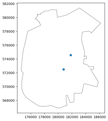
First of all, let us subset the towns layer to retain just the Beer-Sheva shapely polygon, as follows:
pol = towns[towns['Muni_Heb'] == 'באר שבע']
pol = pol.geometry.iloc[0]
pol

Now, let’s evaluate the intersection between each geometry in stations, on the one hand, and the individual pol geometry, on the other hand, using the .intersects method:
sel = stations.intersects(pol)
sel
0     False
1     False
2     False
3     False
4     False
      ...
58    False
59     True
60    False
61    False
62    False
Length: 63, dtype: bool
The result sel is a boolean Series, indicating for each stations feature whether it intersects with the Beer-Sheva polygon.
Exercise 09-e
How can we check how many of the
stationsfeatures intersect with the polygon, i.e., to count the number ofTruevalues in theselseries?
Using the boolean Series from the previous code section, we can subset (see DataFrame filtering) the railway stations that are within Beer-Sheva:
stations[sel]
| STAT_NAMEH | OFF_7_DAY | geometry | nearest_seg_dist | nearest_seg_name | |
|---|---|---|---|---|---|
| 41 | באר שבע מרכז | 174.0 | POINT (180768.91 572476.735) | 34.113422 | באר שבע אוניברסיטה - באר שבע |
| 59 | באר שבע אוניברסיטה | 130.0 | POINT (181813.614 574550.411) | 7.540327 | באר שבע צפון - באר שבע אוניב |
Here is the plot of the resulting stations subset, on top of the town polygon used for filtering them:
base = gpd.GeoSeries(pol).plot(color='none', edgecolor='grey')
stations[sel].plot(ax=base);
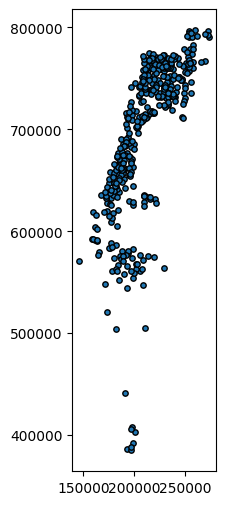
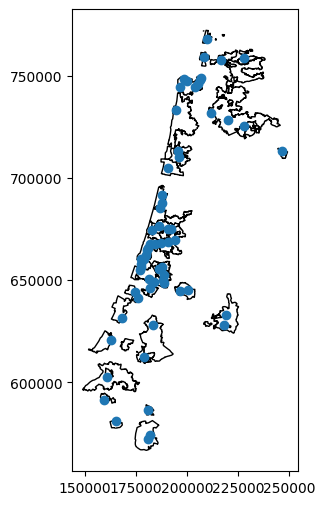
Another common scenarion is when we want to subset by location based on an entire layer, rather than one specific geometry. For example, suppose that we want to select all towns that have at least one railway station. To do that, we can “dissolve” the stations layer using .union_all:
pnt = stations.union_all()
pnt

and then use it for subsetting through .intersects:
towns1 = towns[towns.intersects(pnt)]
towns1
| Muni_Heb | geometry | Machoz | area_km2 | |
|---|---|---|---|---|
| 4 | אופקים | POLYGON Z ((164806.146 577898.8... | דרום | 16.352399 |
| 16 | אשדוד | POLYGON Z ((168551.19 631688.68... | דרום | 63.921935 |
| 18 | אשקלון | POLYGON Z ((161804.408 617717.9... | דרום | 52.318022 |
| 21 | באר יעקב | MULTIPOLYGON Z (((186344.49 651... | מרכז | 9.460773 |
| 22 | באר שבע | POLYGON Z ((175342.311 568405.3... | דרום | 117.393493 |
| ... | ... | ... | ... | ... |
| 261 | רחובות | POLYGON Z ((182522.016 647565.9... | מרכז | 23.757677 |
| 264 | רמלה | POLYGON Z ((187465.305 649941.0... | מרכז | 13.388352 |
| 272 | שדות דן | POLYGON Z ((185799.044 652407.8... | מרכז | 29.346022 |
| 278 | שער הנגב | POLYGON Z ((173176.919 603057.4... | דרום | 176.157893 |
| 281 | תל אביב - יפו | POLYGON Z ((186077.611 668970.3... | תל אביב | 57.096655 |
40 rows × 4 columns
The following figure shows the selected towns:
base = towns1.plot(color='none', edgecolor='black')
stations.plot(ax=base);
Spatial join#
Ordinary spatial join#
Spatial join merges two spatial layers, in the same sense that an ordinary (i.e., non-spatial) join merges two tables (see Joining tables). The difference is that matching rows (i.e., features) are not determined according to identical values in a shared column. Instead, they are determined based on spatial relations. Typically, spatial join is based on the intersection relation (see Boolean methods (geopandas)), meaning that we are joining attributes of feature(s) from the second layer, which intersect with the given feature in the first layer.
In geopandas, spatial join is done using the gpd.sjoin (“spatial join”) function. The gpd.sjoin function takes the following arguments:
left_df—The first (“left”) layerright_df—The second (“right”) layerhow—The type of join, one of:'inner'(the default)'left''right'
predicate—The spatial relation to evaluate when looking for a match, one of:'intersects'(the default)'contains''crosses''overlaps''touches''within'
You may notice similarities with the pd.merge function for ordinary (non-spatial) join (see Joining tables). Namely, three of the four parameters are the same: the two tables/layers, and the how argument for join type. The difference is just the method for evaluating the matching rows/features:
In an ordinary join, matching rows are determined based on identical values in common column(s), specified using the
onargument ofpd.mergeIn a spatial join, matching features are determined based on spatial relations, such as whether the two features intersect or not, whereas the type of relation is specified using the
predicateargument ofgpd.sjoin
For example, the following spatial join operation reveals, for each railway station, which town it intersects with (i.e., located within). We also limit the input layers to just one attribute each, to see more clearly what is going on:
gpd.sjoin(
    stations[['STAT_NAMEH', 'geometry']],
    towns[['Muni_Heb', 'geometry']],
    how='left'
)
| STAT_NAMEH | geometry | index_right | Muni_Heb | |
|---|---|---|---|---|
| 0 | ראשון לציון משה דיין | POINT (177206.094 655059.936) | 258 | ראשון לציון |
| 1 | קרית ספיר נתניה | POINT (187592.123 687587.598) | 213 | נתניה |
| 2 | ת"א השלום | POINT (180621.94 664537.21) | 281 | תל אביב - יפו |
| 3 | שדרות | POINT (160722.849 602798.889) | 278 | שער הנגב |
| 4 | רמלה | POINT (188508.91 648466.87) | 264 | רמלה |
| ... | ... | ... | ... | ... |
| 58 | מגדל העמק כפר ברוך | POINT (219851.931 728164.825) | 227 | עמק יזרעאל |
| 59 | באר שבע אוניברסיטה | POINT (181813.614 574550.411) | 22 | באר שבע |
| 60 | חיפה בת גלים | POINT (198610.01 748443.79) | 81 | חיפה |
| 61 | לוד | POINT (188315.977 650289.373) | 123 | לוד |
| 62 | נהריה | POINT (209570.59 767769.22) | 204 | נהריה |
63 rows × 4 columns
The spatial join result contains the attributes and geometry of the left layer, plus joined attributes and indices ('index_right') of the right layer. In this case, we have:
the
'STAT_NAMEH','geometry'columns from the “left”stationslayer, andthe
'index_right'and'Muni_Eng'columns joined from the “right”townslayer.
For example, the first feature in the spatial join result reveals that the 'ראשון לציון משה דיין' station is located in the town 'ראשון לציון'.
As another, more complicated, example, the following spatial join might be a first attempt to can check which railway segment goes through each railway station:
gpd.sjoin(
    stations[['STAT_NAMEH', 'geometry']],
    rail,
    how='left'
)
| STAT_NAMEH | geometry | index_right | SEGMENT | length_km | |
|---|---|---|---|---|---|
| 0 | ראשון לציון משה דיין | POINT (177206.094 655059.936) | NaN | NaN | NaN |
| 1 | קרית ספיר נתניה | POINT (187592.123 687587.598) | NaN | NaN | NaN |
| 2 | ת"א השלום | POINT (180621.94 664537.21) | NaN | NaN | NaN |
| 3 | שדרות | POINT (160722.849 602798.889) | NaN | NaN | NaN |
| 4 | רמלה | POINT (188508.91 648466.87) | NaN | NaN | NaN |
| ... | ... | ... | ... | ... | ... |
| 58 | מגדל העמק כפר ברוך | POINT (219851.931 728164.825) | NaN | NaN | NaN |
| 59 | באר שבע אוניברסיטה | POINT (181813.614 574550.411) | NaN | NaN | NaN |
| 60 | חיפה בת גלים | POINT (198610.01 748443.79) | NaN | NaN | NaN |
| 61 | לוד | POINT (188315.977 650289.373) | NaN | NaN | NaN |
| 62 | נהריה | POINT (209570.59 767769.22) | NaN | NaN | NaN |
63 rows × 5 columns
In this case, we see that none, or at least the first and last few, stations, had a match. This means that none of the lines precisely intersect with the station points.
One way to overcome this is to use nearest-neighbor join (see Nearest neighbor join). Another option is to use a buffered version of the stations, say with a 100 \(m\) buffer. In this case, we join the attributes of the segments that are within a 100 \(m\) distance from each station:
stations1 = stations.copy()
stations1.geometry = stations1.buffer(100)
stations1[['STAT_NAMEH', 'geometry']]
| STAT_NAMEH | geometry | |
|---|---|---|
| 0 | ראשון לציון משה דיין | POLYGON ((177306.094 655059.936... |
| 1 | קרית ספיר נתניה | POLYGON ((187692.123 687587.598... |
| 2 | ת"א השלום | POLYGON ((180721.94 664537.21, ... |
| 3 | שדרות | POLYGON ((160822.849 602798.889... |
| 4 | רמלה | POLYGON ((188608.91 648466.87, ... |
| ... | ... | ... |
| 58 | מגדל העמק כפר ברוך | POLYGON ((219951.931 728164.825... |
| 59 | באר שבע אוניברסיטה | POLYGON ((181913.614 574550.411... |
| 60 | חיפה בת גלים | POLYGON ((198710.01 748443.79, ... |
| 61 | לוד | POLYGON ((188415.977 650289.373... |
| 62 | נהריה | POLYGON ((209670.59 767769.22, ... |
63 rows × 2 columns
Then, we join the buffered stations1 with the rail layer:
gpd.sjoin(
    stations1[['STAT_NAMEH', 'geometry']],
    rail,
    how='left'
)
| STAT_NAMEH | geometry | index_right | SEGMENT | length_km | |
|---|---|---|---|---|---|
| 0 | ראשון לציון משה דיין | POLYGON ((177306.094 655059.936... | 81.0 | משה דיין-חולות_82 | 1.851570 |
| 0 | ראשון לציון משה דיין | POLYGON ((177306.094 655059.936... | 22.0 | משה דיין-קוממיות_23 | 1.477394 |
| 1 | קרית ספיר נתניה | POLYGON ((187692.123 687587.598... | 100.0 | נתניה מכללה - נתניה ספיר_101 | 1.417325 |
| 2 | ת"א השלום | POLYGON ((180721.94 664537.21, ... | 79.0 | יצחק שדה - השלום_80 | 1.009135 |
| 2 | ת"א השלום | POLYGON ((180721.94 664537.21, ... | 57.0 | סבידור מרכז - השלום_58 | 1.286116 |
| ... | ... | ... | ... | ... | ... |
| 60 | חיפה בת גלים | POLYGON ((198710.01 748443.79, ... | 153.0 | חוף כרמל - בת גלים_156 | 6.121700 |
| 60 | חיפה בת גלים | POLYGON ((198710.01 748443.79, ... | 193.0 | השמונה - בת גלים_197 | 1.644544 |
| 61 | לוד | POLYGON ((188415.977 650289.373... | 77.0 | לוד - רמלה_78 | 1.339807 |
| 61 | לוד | POLYGON ((188415.977 650289.373... | 198.0 | לוד-רמלה מערב_203 | 1.412130 |
| 62 | נהריה | POLYGON ((209670.59 767769.22, ... | NaN | NaN | NaN |
113 rows × 5 columns
In this case, there are even stations with more than one matching line (e.g., 'ראשון לציון משה דיין'), because there can be more than one railway segment passing through a radius of 100 \(m\) of a railway station. However, other stations still had zero matches (e.g., 'נהריה'). This leads us to the second option of dealing with the situation, the nearest neighbor join (see below, Nearest neighbor join).
Exercise 09-f
Note that the last station (
'נהריה') has “No Data” in the segment name column ('SEGMENT'). Can you explain why?
Nearest neighbor join#
In addition to spatial join based on “ordinary” relations such as intersection (see Ordinary spatial join), the geopandas package also has a gpd.sjoin_nearest function for spatial join based on nearest neighbors. It works similarly to gpd.sjoin, but matches are determined based on shortest pairwise distance.
The following expression joins the nearest railway line attributes (including segment name, 'SEGMENT') and specifies the distances in the 'dist' column as requested using the distance_col='dist' argument:
stations = gpd.sjoin_nearest(
    stations[['STAT_NAMEH', 'nearest_seg_dist', 'nearest_seg_name', 'geometry']],
    rail[['SEGMENT', 'geometry']],
    distance_col='dist'
)
stations
| STAT_NAMEH | nearest_seg_dist | nearest_seg_name | geometry | index_right | SEGMENT | dist | |
|---|---|---|---|---|---|---|---|
| 0 | ראשון לציון משה דיין | 13.440327 | משה דיין-קוממיות_23 | POINT (177206.094 655059.936) | 22 | משה דיין-קוממיות_23 | 13.440327 |
| 1 | קרית ספיר נתניה | 4.932094 | נתניה מכללה - נתניה ספיר_101 | POINT (187592.123 687587.598) | 100 | נתניה מכללה - נתניה ספיר_101 | 4.932094 |
| 2 | ת"א השלום | 16.180832 | סבידור מרכז - השלום_58 | POINT (180621.94 664537.21) | 57 | סבידור מרכז - השלום_58 | 16.180832 |
| 3 | שדרות | 64.381044 | שדרות-יד מרדכי_134 | POINT (160722.849 602798.889) | 131 | שדרות-יד מרדכי_134 | 64.381044 |
| 4 | רמלה | 2.941401 | לוד - רמלה_88 | POINT (188508.91 648466.87) | 87 | לוד - רמלה_88 | 2.941401 |
| ... | ... | ... | ... | ... | ... | ... | ... |
| 58 | מגדל העמק כפר ברוך | 56.102377 | עפולה - כפר ברוך_155 | POINT (219851.931 728164.825) | 152 | עפולה - כפר ברוך_155 | 56.102377 |
| 59 | באר שבע אוניברסיטה | 7.540327 | באר שבע צפון - באר שבע אוניב | POINT (181813.614 574550.411) | 205 | באר שבע צפון - באר שבע אוניב | 7.540327 |
| 60 | חיפה בת גלים | 44.130049 | חוף כרמל - בת גלים_156 | POINT (198610.01 748443.79) | 153 | חוף כרמל - בת גלים_156 | 44.130049 |
| 61 | לוד | 22.556829 | לוד - רמלה_78 | POINT (188315.977 650289.373) | 77 | לוד - רמלה_78 | 22.556829 |
| 62 | נהריה | 115.502833 | נהריה - עכו_13 | POINT (209570.59 767769.22) | 12 | נהריה - עכו_13 | 115.502833 |
63 rows × 7 columns
This time, we get exactly one matching rail segment per stations point. In addition to the segment name ('SEGMENT'), the distance to the matched nearest segment is documented in the 'dist' column. As you can see, the values in these two columns are identical to the 'nearest_seg_name' and 'nearest_seg_dist' columns, respectively, which we calculated earlier using a “manual” approach (see Nearest neighbors):
(stations['nearest_seg_name'] == stations['SEGMENT']).all()
np.True_
(stations['nearest_seg_dist'] == stations['dist']).all()
np.True_
Note
For more information, see the gpd.sjoin_nearest function documentation: https://geopandas.org/en/stable/docs/reference/api/geopandas.sjoin_nearest.html.
More exercises#
Exercise 09-g
Read the towns (
'muni_il.shp') layer (see Sample data)Aggregate it according to the
'Machoz'column to dissolve the towns into district polygons (see Dissolving by district)Calculate the number of neighbors, i.e., districts it intersects with excluding self, that each district has.
Plot the result (Fig. 58).
Advanced: display labels with the number of neighbors per district (Fig. 58), by adapting this StackOverflow answer.
Hint:
Join the layer with itself, based on ‘intersection’, to join each town with all of its neighbors, then use aggregation to calculate the sum of joined towns per town. You can create a
'count'variable for each town, equal to1, then sum it when calculating the number of neighbors.Subtract
1to get the number of intersections excluding intersection with self, i.e., the number of neighbors.
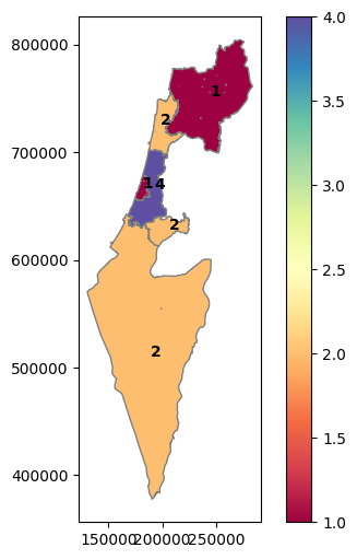
Fig. 58 Solution of exercise-09-g: Neighbor count per town#
Exercise 09-h
Calculate the total population size in a 1 \(km\) buffer around each railway station in
'RAIL_STAT_ONOFF_MONTH.shp', according to the population data in'statisticalareas_demography2019.gdb'('Pop_Total'=total population).Sort the table, to see which stations are situated in the most dense and sparse areas (Fig. 59).
Go through the following steps:
Import both layers into
GeoDataFrameobjectsCalculate the area of each statistical area polygon
Fill the missing population estimates (in the
'Pop_Total'column) with zerosCreate a buffer of 1 \(km\) around the station points
Calculate a layer of pairwise intersections between the buffers and the statistical areas
Calculate the area of each intersection
Calculate the population count of each intersection. To do that, multiply the statistical area population count column (
'Pop_Total') by the ratio between the intersection area, and the original total area of that statistical area (which you calculated in the second step earlier).Aggregate the layer by rail station name, to calculate the total population count per 1 \(km\) buffer around a station
Sort the layer by population counts, to see which stations are situated in the most dense and sparse areas
| STAT_NAMEH | geometry | pop1 | |
|---|---|---|---|
| 11 | בת ים יוספטל | POLYGON ((177152.75 657153.746,... | 55761.058635 |
| 24 | ירושלים יצחק נבון | POLYGON ((218650.757 632087.423... | 46441.448009 |
| 62 | ת"א סבידור מרכז | POLYGON ((180306.847 665089.717... | 39493.940946 |
| 16 | חולון וולפסון | POLYGON ((176806.558 659551.427... | 35295.776253 |
| 48 | קרית מוצקין | POLYGON ((206654.795 747716.12,... | 35148.940155 |
| ... | ... | ... | ... |
| 32 | מגדל העמק כפר ברוך | POLYGON ((218894.991 727874.541... | 29.732200 |
| 23 | יקנעם כפר יהושוע | POLYGON ((212300.18 731084.998,... | 0.000000 |
| 17 | חוצות המפרץ | POLYGON ((205604.63 745103.145,... | 0.000000 |
| 42 | פאתי מודיעין | POLYGON ((197394.885 644447.483... | 0.000000 |
| 49 | קרית מלאכי יואב | POLYGON ((184266.43 628244.915,... | 0.000000 |
63 rows × 3 columns
Fig. 59 Solution of exercise-09-h: Railway stations with largest and smallest population counts in a 1 km buffer#
Exercise 09-i
Read the following vector layers (see Sample data):
'muni_il.shp'—Towns'RAIL_STRATEGIC.shp'—Railway lines
Aggregate the towns layer according to the
'Muni_Heb'column to dissolve the separate polygons per town (see Aggregation (.dissolve))Subset only the active railway lines, i.e., where the value in the
'ISACTIVE'column is equal to'פעיל'(see Filtering by attributes)Subset the town polygons that a railway line goes through
Plot the resulting subset of towns and the active railway lines together (Fig. 60)
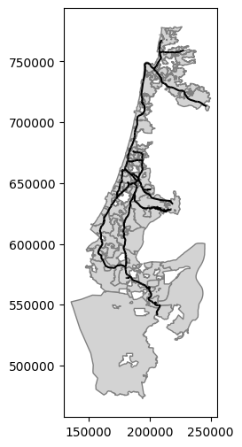
Fig. 60 Solution of exercise-09-i: Towns (grey polygons) intersecting with active railway lines (black lines)#
Exercise 09-j
Read the following vector layers (see Sample data):
'muni_il.shp'—Towns'RAIL_STRATEGIC.shp'—Railway lines
Aggregate the towns layer according to the
'Muni_Heb'column to dissolve the separate polygons per town (see Aggregation (.dissolve))Subset only the active railway lines, i.e., where the value in the
'ISACTIVE'column is equal to'פעיל'(see Filtering by attributes)Calculate and plot the density (\(km / km^2\)) of railway lines per town (Fig. 61)
Print the information for five towns with the highest densities (Fig. 62)
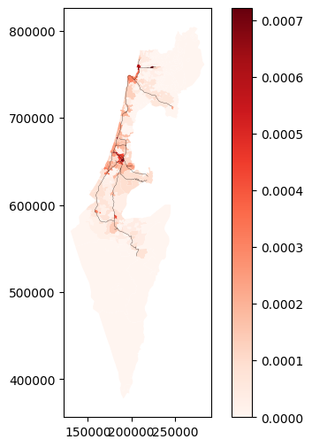
Fig. 61 Solution of exercise-09-j1: Density of active railway lines (black lines) in each town#
| Muni_Heb | geometry | length | area | density | |
|---|---|---|---|---|---|
| 178 | מג'ד אל כרום | POLYGON Z ((217664.43 757558.83... | 6708.740078 | 9.306777e+06 | 0.000721 |
| 123 | לוד | POLYGON Z ((190500.083 653157.0... | 9380.882915 | 1.478579e+07 | 0.000634 |
| 118 | כפר שמריהו | POLYGON Z ((183034.588 677872.3... | 1667.309175 | 2.728429e+06 | 0.000611 |
| 160 | ללא שיפוט - אזור מקווה ישראל - ... | POLYGON Z ((183642.638 658968.6... | 4454.321971 | 7.645018e+06 | 0.000583 |
| 223 | עכו | POLYGON Z ((210673.625 758793.3... | 9865.824430 | 1.809508e+07 | 0.000545 |
Fig. 62 Solution of exercise-09-j2: The five towns with the highest railway line densities#
Exercise solutions#
Exercise 09-b#
import geopandas as gpd
towns = gpd.read_file('data/muni_il.shp', encoding='utf-8')
towns = towns[['Muni_Heb', 'geometry']]
towns['area'] = towns.area
towns1 = towns.sort_values('area')
towns1['Muni_Heb'].iloc[0]
towns1['Muni_Heb'].iloc[towns1.shape[0]-1]
Exercise 09-c#
import geopandas as gpd
towns = gpd.read_file('data/muni_il.shp', encoding='utf-8')
towns = towns[['Muni_Heb', 'Shape_Area', 'geometry']]
towns['area_km2'] = towns.area / 1000**2
towns.plot.scatter('area_km2', 'Shape_Area');
Exercise 09-g#
import geopandas as gpd
# Read data & subset columns
towns = gpd.read_file('data/muni_il.shp', encoding='utf-8')
towns = towns[['Machoz', 'geometry']]
# Dissolve
districts = towns.dissolve(by='Machoz').reset_index()
# Add 'count' variable
districts['count'] = 1
# Spatial join with self
districts = gpd.sjoin(
    districts[['Machoz', 'geometry']],
    districts[['count', 'geometry']],
    how='left',
    predicate='intersects'
)
districts = districts.drop('index_right', axis=1)
# Aggregate
districts = districts.dissolve(by='Machoz', aggfunc='sum')
# Subtract 1 (self)
districts['count'] = districts['count'] - 1
# Plot
districts.plot(column='count', cmap='Spectral', edgecolor='grey', legend=True);
Exercise 09-h#
import pandas as pd
import geopandas as gpd
# Read & subset columns
stations = gpd.read_file('data/RAIL_STAT_ONOFF_MONTH.shp')
stat = gpd.read_file('data/statisticalareas_demography2019.gdb')
stations = stations[['STAT_NAMEH', 'geometry']]
stat = stat[['SHEM_YISHUV', 'Pop_Total', 'geometry']]
# Calculate area
stat['area'] = stat.area
# Replace "No Data" population with 0
stat['Pop_Total'] = stat['Pop_Total'].fillna(0)
# Buffer stations
stations.geometry = stations.buffer(1000)
# Intersect
stations = gpd.overlay(stations, stat, how="intersection")
# Calculate population per polygon
stations['area1'] = stations.area
stations['prop'] = stations['area1'] / stations['area']
stations['pop1'] = stations['Pop_Total'] * stations['prop']
# Dissolve
stations = stations[['STAT_NAMEH', 'pop1', 'geometry']].dissolve(by='STAT_NAMEH', aggfunc='sum').reset_index()
# Sort
stations = stations.sort_values(by='pop1', ascending=False)
stations