Arrays (numpy)

Last updated: 2024-03-29 20:03:58

---

Introduction

Arrays are fundamental when working with data. Many types of data are convenient to arrange and represent using arrays, and many types of data processing operations are facilitated through the use of arrays. For example:

• Tables are represented as collections of one-dimensional arrays, having the same length, where each array represents a table column (see Tables (pandas))

• Digital images and spatial rasters are represented with arrays, possibly with spatial metadata (such as the Coordinate Reference System) (see Rasters (rasterio) and Raster-vector interactions)

In this chapter we cover our first third-party package, named numpy. The numpy package deals with arrays. We are going to learn about methods for working with arrays, including:

• Creating arrays

• Subsetting arrays

• Vectorized operations

• Summarizing array values

• Reading array from file

• Plotting (numpy) (using the matplotlib package)

In this chapter we work with the numpy package on its own. However, as we will see in later chapters, the numpy package comprises the foundation for many other data analysis-related domains in Python, inclusing spatial data analysis. For example, table (see Tables (pandas)) and vector layer (see Vector layers (geopandas)) columns, as well as rasters (see Rasters (rasterio)), are internally represented by numpy arrays. Therefore, although the material in this chapter may seem abstract at first, keep in mind that it is going to be practically applicable soon enough, throughout all of the remaining chapters.

What is numpy?

numpy (short for “numerical python”) is a well-established Python package for scientific computing with arrays, and for working with data in general. The numpy package provides standardized data structures, functions, and operators for homogeous arrays, facilitating efficient computation and shorter code. Namely, thanks to the fact that a numpy array is uniform, in terms of data types, processing is much more efficient compared to a list (see Lists (list)). numpy also provides “vectorized” operators for arrays, which otherwise require using for loops (see for loops) or list comprehension (see List comprehension) when working with lists.

Note

NumPy: the absolute basics for beginners is a recommended official overview of numpy.

numpy is a core package in the data science ecosystem of Python, so it is worthwhile to learn it no matter what aspect of data science you are going to explore later on. numpy is the foundation for many other, more specialized, packages in Python, including the main packages we learn about later on in this book:

• pandas for working with tables (see Tables (pandas))

• geopandas for working with vector layers (see Vector layers (geopandas))

• rasterio for working with rasters (see Rasters (rasterio))

Assuming it is installed (see Installing packages), to start working with numpy we first need to import it (see Loading packages). By convention, numpy is imported as np:

import numpy as np

What is an array?

An array is an ordered sequence of values, arranged in an n-dimensional structure. In this book, we are going to focus on the three most useful types of arrays:

• One-dimensional—A sequence of values, analogous to a “flat” (i.e., non-hierarchical) list

• Two-dimensional—A matrix, i.e., a collection of sequences, all of the same length, arranged into a rectangular structure

• Three-dimensional—A “cubic” array, i.e., a collection of matrices of the same size, arranged into layers

Keep in mind that an array can also be:

• 0-dimensional—a single value, such as when extracting an individual element from an array (see Individual values), or

• ≥4-dimensional—high-dimensional arrays, less useful for our purposes (and in general)

In spatial raster terminology (see Rasters (rasterio)),

• a two-dimensional array corresponds to a single-band raster, and

• a three-dimensional array corresponds to a multi-band raster.

In numpy, arrays are represented by a data type called ndarray (short for “N-dimensional array”).

Creating arrays

Overview

An ndarray can be created in several ways, which we demonstrate in this section:

• From a list (see ndarray from list)

• By repeating a sequence (see Using np.tile and Using np.repeat)

• By calculating a consecutive sequence (see Using np.arange and Using np.linspace)

Later on we will demostrate that an array can also be imported from a file, such as a CSV file (see Reading array from file).

ndarray from list

In case we wish to manually specify all of the array values, the np.array function can be used to convert a list into an array. For example, a flat list can be converted to a one-dimensional array, hereby named a, as follows:

a = np.array([3, 8, -2, 43, 12, 1, 8])
a

array([ 3,  8, -2, 43, 12,  1,  8])

A “nested” list, i.e., a list of lists, can be converted to a two-dimensional array, where the internal lists comprise the rows, hereby named b:

b = np.array([[1, 0, 0], [2, 1, 2], [3, 1, 0], [2, np.nan, 1]])
b

array([[ 1.,  0.,  0.],
       [ 2.,  1.,  2.],
       [ 3.,  1.,  0.],
       [ 2., nan,  1.]])

Note that array b contains a special value np.nan, which represents “No Data”, i.e., an unknown value in the array. We will elaborate on how np.nan values are treated in various operations, later on (see Working with missing data (numpy)). For now, you can get an impression of the np.nan behavior, and start getting used to the possibility of having missing values in a numpy array.

Let us also create a three-dimensional array named c. Rather than typing all values manually, here we are using the np.arange function and the .reshape function, which we will explain later on (see Using np.arange and General reshaping (.reshape), respectively). What is important, for now, is that the resulting object is a three-dimensional array:

c = np.arange(1, 25).reshape((2, 3, 4))
c

array([[[ 1,  2,  3,  4],
        [ 5,  6,  7,  8],
        [ 9, 10, 11, 12]],

       [[13, 14, 15, 16],
        [17, 18, 19, 20],
        [21, 22, 23, 24]]])

Note that the type of a, b and c, is ndarray:

type(a), type(b), type(c)

(numpy.ndarray, numpy.ndarray, numpy.ndarray)

Using np.tile

Repetitive arrays can be created using the np.tile function, which accepts:

• A—A number, list, or array to repeat

• reps—How many times to repeat it?

For example:

np.tile(12, 7)  ## '12' seven times

array([12, 12, 12, 12, 12, 12, 12])

np.tile([1, 2], 3)  ## '[1,2]' three times

array([1, 2, 1, 2, 1, 2])

np.tile(a, 2)  ## 'a' two times

array([ 3,  8, -2, 43, 12,  1,  8,  3,  8, -2, 43, 12,  1,  8])

Using np.repeat

There is another function, named np.repeat, for creating repetitive arrays. Unlike np.tile, the np.repeat function repeats each element consecutively and not the entire array (or list). Compare the following example with np.tile([1,2],3) (Using np.tile):

np.repeat([1, 2], 3)

array([1, 1, 1, 2, 2, 2])

Using np.arange

It is often useful to create sequential arrays. The np.arange function can be used to create sequential arrays, given:

• start—The start value

• stop—The end value

• step—The step size

The np.arange function is very similar, in terms of its design, to the range function (see The range function).

For example, the following expression creates an array starting from 5, ending before 12, with step size 1.5:

np.arange(5, 12, 1.5)

array([ 5. ,  6.5,  8. ,  9.5, 11. ])

The default value for step is 1, as demonstrated in the following expression, where we omit step:

np.arange(5, 12)

array([ 5,  6,  7,  8,  9, 10, 11])

When passing a single argument to np.arange, that argument is treated it as stop, whereas the default start is 0 and the default step is 1:

np.arange(12)

array([ 0,  1,  2,  3,  4,  5,  6,  7,  8,  9, 10, 11])

Using np.linspace

Another useful method to create sequential arrays is np.linspace (short for “linear space”). It accepts three arguments:

• start—The start value

• stop—The end value

• num—Number of points (default is 50)

The np.linspace function then returns evenly spaced points, in the interval specified by start and stop. The step size is automatically calculated to accommodate the specified number of points (default is 50).

For example, the following expression creates a sequence of 9 equally spaced points, between 0 and 4.

np.linspace(0, 4, 9)

array([0. , 0.5, 1. , 1.5, 2. , 2.5, 3. , 3.5, 4. ])

Note

There are several other functions to facilitate creation of arrays, such as functions to create repetitive arrays:

• np.zeros—Array of given shape filled with 0

• np.ones—Array of given shape filled with 1

• np.full—Array of given shape filled with user-specified value

and functions to create random number arrays, such as:

• np.random.random—Array of given shape filled with random numbers in the interval [0.0, 1.0)

• np.random.normal—Array of given shape filled with random numbers from a normal distribution

• np.random.randint—Array of given shape filled with random integers in the specified interval

Array dimensions

The most basic property of arrays is their shape: the size of each array dimension. This can be accessed using the .shape property. The returned object is a tuple (see Tuples (tuple)), with length according to the number of dimensions:

a.shape

(7,)

b.shape

(4, 3)

c.shape

(2, 3, 4)

A derived property of .shape is the number of dimensions .ndim, which is equal to the “length” of the .shape property:

a.ndim

1

b.ndim

2

c.ndim

3

Another derived property of .shape is the number of elements .size, which is equal to a multiplication of all dimension lengths:

a.size

7

b.size

12

c.size

24

At this point, you may wonder what is the reason for using an array rather than simply a list. This leads us to the main difference between arrays and lists: the fact that an array, unlike a list, is composed of values of the same type. This makes arrays more restrictive than lists, but also much more efficient in terms of storage size and computation speed.

Data types

Checking data type

As mentioned above, ndarray objects are composed of values of the same type. We can check the type of an existing array using the .dtype (“data type”) property. For example:

a.dtype

dtype('int64')

b.dtype

dtype('float64')

The above printout means that a is an integer array, while b is a float array. You can also see that numpy accommodates more detailed distinction between data types than basic Python, with integer and float varieties according to specific precision. For example, int64 and float64 mean 64-bit precision integer and float arrays, respectively (numpy array data types).

The required data type can be specified when constructing an array, using the dtype parameter. The value can be specified using the respective object representing each data type (see numpy array data types). For example:

x = np.array([1, 1, 1], dtype=np.float32)
x

array([1., 1., 1.], dtype=float32)

Note

The int64 and float64 data types in numpy are considered “standard”. Therefore, when printing an array object, the data type specification appears for all data types except for those. Try printing a and b to see for yourself.

Commonly used data types in numpy are summarized in Table 12. As you can see, there are many varieties of numeric types in numpy. This may seem confusing, compared to basic Python or other programming languages such as R, which have just one data type for integer and one for float. However, keep in mind that the purpose of having many specific data types is conserving memory and making calculations more efficient. In practice, int64 and float64 are most commonly used to represent int and float, respectively.

Table 12 numpy array data types

Data type	Description	GeoTIFF
np.bool_/bool	Boolean (True or False) stored as a byte
np.int_/int	Default integer type, normally int64
np.int8	Integer a single byte (-128–127)
np.int16	Integer 16 bits (-32768–32767)	+
np.int32	Integer 32 bits (-2147483648–2147483647)	+
np.int64	Integer 64 bits (-9223372036854775808–9223372036854775807)
np.uint8	Unsigned integer 8 bits (0–255)	+
np.uint16	Unsigned integer 16 bits (0–65535)	+
np.uint32	Unsigned integer 32 bits (0–4294967295)	+
np.uint64	Unsigned integer 64 bits (0–18446744073709551615)
np.float_/float	Default float type, normally float64
np.float16	Half-precision (16 bit) float (-65504–65504)
np.float32	Single-precision (32 bit) float (1e-38–1e38)	+
np.float64	Double-precision (64 bit) float (1e-308–1e308)	+

Note

As a rule of thumb, int arrays should be preferred for integer-only data, since the int data types are capable of exactly representing all of the values in their respective range. float arrays should be used when the data contain decimal parts, or when native representation of “No Data” is required (see Working with missing data (numpy)), but you should be aware that very large numbers are not representable exactly in a float.

numpy also supports creating arrays of “customized” types, and even arrays that do not conform to any of the built-in data types. The latter means that you can create an array where the elements are any type of Python object. Accordingly, the dtype of the resulting array will be object.

For example, the following array of strings has dtype of '<U5', namely “unicode string of length 5”:

s = np.array(['John', 'James', 'Bob'])
s

array(['John', 'James', 'Bob'], dtype='<U5')

An array of dictionaries, however, results in dtype of object, because there is no built-in data type to represent an array of dict elements in numpy:

s = np.array([{'a': 1}, {'b': 2}])
s

array([{'a': 1}, {'b': 2}], dtype=object)

In practice, an array of type “object” implies that processing the array is going to employ “general” Python functions, rather than optimized numpy functions, which is less efficient.

Changing data type

If necessary, an array can be transformed from one data type to another, using the .astype method. The argument of .astype is one of the numpy data types (Table 12). For example, here is how we can transform array a from int64 to float64:

a = a.astype(np.float64)
a

array([ 3.,  8., -2., 43., 12.,  1.,  8.])

Here is how we can transform a to np.int8:

a = a.astype(np.int8)
a

array([ 3,  8, -2, 43, 12,  1,  8], dtype=int8)

and here we go back to int64:

a = a.astype(np.int64)
a

array([ 3,  8, -2, 43, 12,  1,  8])

Keep in mind that:

• We must choose a data type which encompasses the entire range of values in the array (see Table 12). Otherwise, we get meaningless (random) values instead of those beyond the valid range.

• A float type must be used whenever the array contains np.nan values (see “No Data” representation)

Also note that numpy defines special data types np.int_ and np.float_, which refer to “default” int and float data types. These are platform dependent, but typically resolve to np.int64 and np.float64 (numpy array data types). Furthermore, the standard Python types int and float (Numbers (int, float)) refer to those two numpy types, respectively. Therefore, for example, either of the three objects np.int64, np.int_ and int can be passed to .astype in the above example, with identical result. In practice, we will use the shorter int:

a = a.astype(int)
a

array([ 3,  8, -2, 43, 12,  1,  8])

Subsetting arrays

Overview

Array subsets are created by passing indices, separated by commas, inside square brackets ([). The number of indices needs to be in agreement with the number of dimensions. The order of array dimensions (and indices) is:

• array[rows,columns]—for a two-dimensional array

• array[layers,rows,columns]—for a three-dimensional array

The indices start from 0, like in other Python data structures (see Accessing list elements).

Individual values

For example, here is how we can get individual elements out of an array:

a[1]        ## 2nd element

8

b[1, 2]     ## Element in 2nd row, 3rd column

2.0

c[1, 0, 3]  ## Element in 2nd layer, 1st row, 4th column

16

When subsetting individual values from an array, we get a plain numpy value, such as an int64 or float64. Technically speaking, the result is simplified to a zero-dimensional numpy array:

type(a[1])

numpy.int64

Array slices

Any of the indices can be replaced with :, which means “return all subsets in that dimension”. For example:

b[1, :]  ## 2nd row, all columns

array([2., 1., 2.])

b[:, 1]  ## 2nd column, all rows

array([ 0.,  1.,  1., nan])

c[:, 2, :]  ## 3rd row, all layers and all columns

array([[ 9, 10, 11, 12],
       [21, 22, 23, 24]])

We can also assign new values into an individual element, or a slice, of an array, in which case the respective elements are replaced. Try this for yourself to see how it works.

Exercise 04-a

• How many dimensions does c[1,2,:] have?

• What about c[1,:,:]?

• Check your answers using an expression which returns the number of dimensions.

The start:stop notation which we learned about for list subsetting (see list slicing) is applicable to numpy arrays too. For example:

b[:2, :]  ## 1st and 2nd rows

array([[1., 0., 0.],
       [2., 1., 2.]])

b[2:, :]  ## 3rd row and onward

array([[ 3.,  1.,  0.],
       [ 2., nan,  1.]])

b[1:3, :]  # 2nd and 3rd rows

array([[2., 1., 2.],
       [3., 1., 0.]])

When using individual indices, the result is simplified in terms of the number of dimensions. For example, b[:,1] is a one-dimensional array, with the values of one column of a two-dimensional array. When using slices, however, the result is never simplified, even the slice refers to just one element along the dimension. For example, compare the following methods to subset the second column of b:

b[:, 1]    ## Subset 2nd column using individual index

array([ 0.,  1.,  1., nan])

b[:, 1:2]  ## Subset 2nd column using slice

array([[ 0.],
       [ 1.],
       [ 1.],
       [nan]])

Examples of subsetting a two-dimensional array are visualized in Fig. 23.

Fig. 23 Subsetting a two-dimensional numpy array

Exercise 04-b

• Replace one of the values in the array b with a new value.

• Replace an entire row with a new value.

• Replace an entire column with a new value.

Views and copies (numpy)

A numpy array is a mutable object. In agreement with the basic behavior of mutable objects, such as lists in Python (see Mutability and copies), this means that a copy of the original object is (by default) a reference to the same memory location. Any change we make in such a references is therefore “reflected” in both.

In Mutability and copies, we have seen that assigning a list to another variable creates a reference to the same list. The same behavior takes places with numpy arrays. Moreover, and unlike lists, a subset of a numpy array is also a reference to the original (whereas a list subset is automatically copied). Therefore modifying an array subset is, too, reflected in the original array, unless we explicitly make an independent copy of the array and subset the copy.

Let us demonstrate the behavior described in the last paragraph. Suppose that we take a subset with the 2^nd row from array b and assign it to b1:

b1 = b[1, :]
b1

array([2., 1., 2.])

and then replace one of the values with a different value, such as 999:

b1[1] = 999

As expected, the subset b1 now contains the new value:

b1

array([  2., 999.,   2.])

What may be unexpected, is that the original array b, where the subset comes from, is also updated:

b

array([[  1.,   0.,   0.],
       [  2., 999.,   2.],
       [  3.,   1.,   0.],
       [  2.,  nan,   1.]])

The reason for this behavior is that a subset is not a true copy of the underlying array. Instead, it can be thought of as a view, or reference, to the array, or to a subset of it. Any modification of the “view” modifies the original array as well.

In case we are interested in a “real” copy, which is independent of the original, we must explicitly use the .copy method (see Mutability and copies). For example, let us return b to its original form (again through the view b1!):

b1[1] = 1
b

array([[ 1.,  0.,  0.],
       [ 2.,  1.,  2.],
       [ 3.,  1.,  0.],
       [ 2., nan,  1.]])

Now, let us create a subset which is a copy of b2, and modify it:

b2 = b[1, :].copy()
b2[1] = 999

Again, the subset is modified as expected:

b2

array([  2., 999.,   2.])

The original array b, however, is unchanged, since b2 is an independent copy:

b

array([[ 1.,  0.,  0.],
       [ 2.,  1.,  2.],
       [ 3.,  1.,  0.],
       [ 2., nan,  1.]])

Keep in mind that there are operations other than subsetting that return a “view”, rather than a copy, such as:

• .reshape (see General reshaping (.reshape))

• .T (see Transposing (.T)).

ndarray to list

A numpy array can be converted to a list using the .tolist method. This can be thought of as the opposite creating an array from a list with np.array (see ndarray from list). For example:

b.tolist()

[[1.0, 0.0, 0.0], [2.0, 1.0, 2.0], [3.0, 1.0, 0.0], [2.0, nan, 1.0]]

This may be useful when we prefer to process our data using basic Python functions, rather than numpy functions and methods.

Array reshaping

General reshaping (.reshape)

Array reshaping means transferring the array values to an array with a different shape. Arrays can be reshaped using the .reshape method, which accepts a tuple with the new shape. For example, the following expression transforms the one-dimensional array a with shape (7,) into a two-dimensional array with shape (7,1), i.e., seven rows and one column:

a.reshape((7, 1))

array([[ 3],
       [ 8],
       [-2],
       [43],
       [12],
       [ 1],
       [ 8]])

The following expression transforms b into a two-dimensional array of a different shape, from shape (4,3) to shape (2,6):

b.reshape((2, 6))

array([[ 1.,  0.,  0.,  2.,  1.,  2.],
       [ 3.,  1.,  0.,  2., nan,  1.]])

As mentioned above, .reshape returns a “view” of the original array (see Views and copies (numpy)).

Note

You can use -1 for dimensions in .reshape to be calculated automatically, according to the other dimension(s) and the length of the data. For example, try b.reshape((-1,6)) instead of the last expression.

Note

Another way of reshaping an array, specific to the case where we add a new dimension, is to use np.newaxis. For example, a[:,np.newaxis] and a[np.newaxis,:] transform a into a two-dimensional array with a new length-one dimension of columns or rows, respecively. Try these expressions in the console to see for yourself.

To one-dimensional (.flatten)

A common reshaping operation is “collapsing” a multy-dimensional array into a one-dimensional array. This can be done using the .flatten method:

b.flatten()

array([ 1.,  0.,  0.,  2.,  1.,  2.,  3.,  1.,  0.,  2., nan,  1.])

“Flattening” can be useful when we need to treat all values of a two- (or three-) dimensional array as a single sequence, for example to calculate global statistics, or to display a histogram (see Histograms (numpy)).

Transposing (.T)

Finally, it is often useful to transpose a two-dimensional array, that is, to turn array rows into columns and vice versa. The transposed array is accessible through the .T property:

b

array([[ 1.,  0.,  0.],
       [ 2.,  1.,  2.],
       [ 3.,  1.,  0.],
       [ 2., nan,  1.]])

b.T

array([[ 1.,  2.,  3.,  2.],
       [ 0.,  1.,  1., nan],
       [ 0.,  2.,  0.,  1.]])

Transposing is useful in situations when we need to apply a function that treats array rows and columns differently, such as when plotting (see Line plots (numpy)).

As mentioned above, .T returns a “view” of the original array (see Views and copies (numpy)).

Vectorized operations

Overview

Vectorized operations, also known as “Universal functions” in numpy terminology, make it possible to apply the same operation on all elements of an array at once. Vectorized operations (discussed in this section) and summary functions (see Summarizing array values), are two big advantages and motivations of using numpy, both in terms of shorter code and efficiency, compared to “basic” methods such as lists. Due to their efficient storage, vectorized operations on numpy arrays are much more efficient and fast than, say, a for loop or a list complehension repeatedly performing the same operation on all elements of a list.

There are numerous built-in vectorized operators and functions in numpy, and there are methods to define new ones. The operations are pairwise, element-by-element. We can combine:

• an array with another array (e.g., b+b), or

• an array with an individual number (e.g., b+1).

In the latter case, the number is automatically treated as an array with repeated values.

Arithmetic operators

All arithmetic operators (see Arithmetic operators) are implemented as vectorized numpy operators. Let us take array a as an example:

a

array([ 3,  8, -2, 43, 12,  1,  8])

Here are a few examples of arithmetic array operations:

a + 1     ## Add 1 to elements of 'a'

array([ 4,  9, -1, 44, 13,  2,  9])

-a        ## Inverse of elements 'a'

array([ -3,  -8,   2, -43, -12,  -1,  -8])

a * a     ## Multiply each element of 'a' by itself (same as 'a**2')

array([   9,   64,    4, 1849,  144,    1,   64])

1000 - a  ## Subtract each element in 'a' from 1000

array([ 997,  992, 1002,  957,  988,  999,  992])

Functions on each element

Numerous numpy functions are defined as vectorized functions, to perform an operation on each element, resulting in a new array of exactly the same shape as the input, containing the result. For example, the np.abs function is used to calculate the absolute value of each element in an array:

np.abs(a)

array([ 3,  8,  2, 43, 12,  1,  8])

which is analogous to using basic abs function (see Functions) on plain int or float values.

numpy conditional operators

Python’s conditional operators (see Conditions) are also implemented as vectorized operators in numpy. For example:

a > 10       ## Is each element of 'a' greater than 10?

array([False, False, False,  True,  True, False, False])

a == abs(a)  ## Is each element of 'a' equal to its absolute value?

array([ True,  True, False,  True,  True,  True,  True])

Note that the result of conditional operations on an array is a boolean (see Boolean values (bool)) array, as evident when examining the .dtype property (see Checking data type):

(a > 10).dtype

dtype('bool')

Boolean arrays can be negated with the ~ operator, or combined with & (and) and | (or) operators (Table 13):

• The ~ operator is analogous to not (see Table 10), i.e., it negates a boolean array, replacing True with False and vice versa

• The & operator is analogous to and (see Table 10)

• The | operator is analogous to or (see Table 10)

Remember that &, |, and ~ should be used when working with arrays. The analogous and, or, and not operators which we covered earlier (see Table 10), are applicable to entire objects, not arrays elements.

Table 13 Logical operators for numpy arrays

Operator	Meaning
&	And
|	Or
~	Not

Let us demonstrate the &, |, and ~ operators through examples. First, suppose that we have two boolean arrays, a>5 and a<15:

a > 5

array([False,  True, False,  True,  True, False,  True])

a < 15

array([ True,  True,  True, False,  True,  True,  True])

Here is how they can be combined using the & or the | operator. Beware that you must use parentheses around both sides of the expressions, since &, |, and ~ have higher precedence than comparison operators such as < and >!

(a > 5) & (a < 15)  ## Is each element of 'a' greater than 5 *and* smaller than 15?

array([False,  True, False, False,  True, False,  True])

(a > 5) | (a < 15)  ## Is each element of 'a' greater than 5 *or* smaller than 15?

array([ True,  True,  True,  True,  True,  True,  True])

Here is an example of the ~ operator in action, negating a boolean array:

~(a > 5)  ## Is each element of 'a' *not* greater than 5?

array([ True, False,  True, False, False,  True, False])

Note

Note that in all of the examples in this section which involve two arrays, the arrays had equal dimensions. numpy vectorized operations are, in fact, more general than that. In certain conditions, numpy can accommodate operations between two arrays with different dimensions. This is a powerful technique known as broadcasting. For more details, see https://numpy.org/doc/stable/user/basics.broadcasting.html.

When a boolean array is passed to an arithmetic operation, or function, True values are treated as 1 and False values are treated as 0. The result is then a numeric array. For example, the boolean array a>5:

a > 5

array([False,  True, False,  True,  True, False,  True])

is automatically transformed to a numeric array of 0’s and 1’s when multiplied by 10:

10 * (a > 5)

array([ 0, 10,  0, 10, 10,  0, 10])

Masking

What are masks?

numpy arrays can be subsetted using corresponding boolean arrays, which are also known as masks. Masking is useful for extracting or modifying some of the values in an array—more specifically, those values which correspond to a specified condition. For example, we may want to:

• extract the non-missing values in an array, or

• replace all missing values with a new value, or

• delete (i.e., replace with “No Data”) values that above a particular threshold (e.g., assuming they are measurement errors), and so on.

Any boolean array with a corresponding shape can function as a mask. Typically, a mask is created using a conditional expression (see numpy conditional operators) on the original array itself. For example, given the array named a:

a

array([ 3,  8, -2, 43, 12,  1,  8])

The expression a>10 creates a mask, referring to those elements of a which are greater than 10:

a > 10

array([False, False, False,  True,  True, False, False])

Using masks for subsetting

When passed as an index inside square brackets ([), a mask can be used to filter the array, returning a subset with only those elements that correspond to True. For example:

a[a > 10]

array([43, 12])

Note that when subsetting two- or three-dimensional arrays using a mask, the original shape is not preserved. Instead, the selected values are “collected” into a one-dimensional array. For example:

b[b > 1]

array([2., 2., 3., 2.])

Using masks for assignment

Assignment to a “masked” subset can be used to modify the corresponding subset in the original array. For example, the following expression replaces those values of a which are greater than 10, with a new value 100:

a[a > 10] = 100
a

array([  3,   8,  -2, 100, 100,   1,   8])

The following expression replaces values which are negative or equal to 3 with a new value -99. Again, note the mandatory parentheses.

a[(a < 0) | (a == 3)] = -99
a

array([-99,   8, -99, 100, 100,   1,   8])

Before we move on, let us get back to the original values in array a:

a = np.array([3, 8, -2, 43, 12, 1, 8])
a

array([ 3,  8, -2, 43, 12,  1,  8])

Summarizing array values

Overview

In addition to vectorized, or element-by-element, operations such as np.abs (see Vectorized operations), numpy also accommodates functions to summarize array values, such as np.sum to calculate the array sum. As we will see, there are several modes of operation for summary functions:

• A “global” summary (the default), such as np.sum(x) for the sum of all values in array x

• A summary for subsets along one or more dimensions—using axis=A or axis=(A,B,...), where A, B, etc. are the dimensions being summarized (or “eliminated”), such as np.sum(x,axis=0) for column sums of a two-dimensional array x

The most useful function for summarizing array values, for the purposes of this book, are given in Table 14. Note that some of the functions are defined in two ways:

• as standalone functions (e.g., np.sum)

• as array methods (e.g., .sum)

Both ways are identical, and it is just a matter of preference which one to use. However, standalone functions are accessible more universally:

• Some of the functions only have a standalone version (such as np.median)

• “No Data”-safe functions (such as np.nanmean, see Operations with “No Data”) are only available through standalone functions

Table 14 Commonly used functions to summarize array values in numpy

Operation	Function	Method	“No Data”-safe version
Sum	np.sum	.sum	np.nansum
Minimum	np.min	.min	np.nanmin
Maximum	np.max	.max	np.nanmax
Mean	np.mean	.mean	np.nanmean
Median	np.median	-	np.nanmedian
Index of (first) minimum	np.argmin	.argmin	np.nanargmin
Index of (first) maximum	np.argmax	.argmax	np.nanargmax
Is at least one element True?	np.any	.any	-
Are all elements True?	np.all	.all	-

Global summaries

Unlike vectorized operations (see Vectorized operations), which are performed element-by-element, summary operations return a single result for the entire array (the default), or an array with results for subsets such as the rows and columns. In this section we discuss the former, known as global summaries.

For example, the np.sum function can be used to calculate the global sum of all elements in an array:

np.sum(a)

73

The np.min and np.max functions return the minimum and maximum element, respectively:

np.min(a)

-2

np.max(a)

43

As mentioned above, most numpy summary functions have “method” shortcuts to do the same using shorter code (Table 14). For example, there is a .max method which does the same thing as the np.max function. For example:

a.max()  ## Shortcut to 'np.max(a)'

43

Note

Python has a built-in function called sum, which works on lists as well as numpy arrays. However, sum is much slower, and it is not tailored to numpy arrays, so it is not aware of array dimensions. The same applies to min, max, any, all, and other “base” Python functions. Make sure you are using the specialized numpy functions (such as np.sum) or methods (such as .sum) when working with numpy, to avoid unexpected results!

A common use case of global summary functions is to count True values in a boolean array, typically to find out the number of elements satisfying a given condition. Recall that the arithmetic operators, when applied on a boolean array, treats True values as 1 and False values as 0 (see numpy conditional operators). Therefore, it can be used for “counting” the number of True values. For example:

np.sum(a > 5)   ## How many elements of 'a' are greater than 5?

4

np.sum(a < 15)  ## How many elements of 'a' are smaller than 15?

6

Sometimes we are not interested in the exact number of True values, but rather to figure out if we have at least one True value, or if all values are True. The .any and .all methods used to reveal whether the array contains at least one True, or whether all of its elements are True, respectively. For example:

np.any(a > 5)  ## Is *any* of the elements of 'a' greater than 5?

True

np.all(a > 5)  ## Are *all* elements of 'a' greater than 5?

False

Exercise 04-c

• The np.diff function calculates consecutive differences between elements in an array.

• Write an expression that, using np.diff, checks whether the elements of an array are in increasing order.

• Test your expression using two arrays that are in increasing and non-increasing oderer, such as np.array([2,5,8,9]) and np.array([21,8,9]). The returned values need to be True, and False, respectively.

Summaries per dimension (2D)

As shown above, the default behavior of summary functions, such as np.sum, is to operate on all elements combined (axis=None), resulting in a “global” summary (see Global summaries). Using the axis parameter, however, we can also apply the function on different dimensions, separately.

When referring to two-dimensional arrays, summary functions can be applied separately:

• on each column (axis=0), or

• on each row (axis=1) (Fig. 24).

Fig. 24 Applying a function on each row, or on each column, of a two-dimensional numpy array

Let us demonstrate on the two-dimensional array b:

np.sum(b, axis=0)  ## Column sums

array([ 8., nan,  3.])

np.sum(b, axis=1)  ## Row sums

array([ 1.,  5.,  4., nan])

Note that whenever at least one “No Data” (np.nan) value is passed to np.sum, the result is also “No Data” (Fig. 24). To ignore np.nan values we may use the “No Data”-insensitive version of .sum, namely np.nansum (see Table 14). We elaborate on dealing with “No Data” later on (see Working with missing data (numpy)).

The meaning of the axis parameter can be confusing. To get row-wise summaries (i.e., dimension 0) we are actuially specifying the column dimension (axis=1), and vice versa. Here is how you can remember the meaning of the axis parameter. With the axis parameter, we specify which dimension gets “eliminated” from the resulting array. Accordingly,

• axis=0 “eleminates” dimension 0 (rows), resulting in column-wise summaries

• axis=1 “eliminates” dimension 1 (columns), resulting in row-wise summaries

Summaries per dimension (3D)

Let us now move on to the more complex case of summaries per dimension of three-dimensional arrays. Before we begin, recall that the order of dimensions in a three-dimensional array is (layers,rows,columns) (see Subsetting arrays).

For example, in array c, we have:

• Two “layers”

• Three rows

• Four columns

c.shape

(2, 3, 4)

First, we can get row-wise, column-wise, and “layer”-wise summaries, according to the same principle as with a two-dimensional array (see Summaries per dimension (2D)). We just need to “eliminate” two out of three dimensions, rather than one of two dimensions. In this case, the axis argument is a tuple of length two:

np.sum(c, axis=(1, 2))  ## "Layer" sums

array([ 78, 222])

np.sum(c, axis=(0, 2))  ## Row sums

array([ 68, 100, 132])

np.sum(c, axis=(0, 1))  ## Column sums

array([66, 72, 78, 84])

Second, eliminating one out of three dimensions results in summaries of the two remaining dimensions, which is a little more confusing. Overall, there are three possible combinations of dimension “pairs”:

• axis=0—row-column summaries

• axis=1—column-layer summaries

• axis=2—row-layer summaries

For our purposes in this book, the only useful combination is row-column summaries. In raster terminology, row-column summaries refer to “cell”, or “pixel”, summaries (see Summarizing values). To get row-column summaries, we eliminate the layer dimension:

np.sum(c, axis=0)  ## Row and column (i.e., "pixel") sums

array([[14, 16, 18, 20],
       [22, 24, 26, 28],
       [30, 32, 34, 36]])

Exercise 04-d

• What will be the result of np.argmin(a)? and of np.argmax(a)?

• What will be the result of np.argmax(c, axis=0)?

• What is the meaning of the last result, in plain language?

Working with missing data (numpy)

“No Data” representation

Missing values in a numpy array are typically represented using np.nan (“not a number”), which is a special type of a float value. For example:

x = np.array([1, np.nan, 3])
x

array([ 1., nan,  3.])

Due to the way that numbers are stored in computer memory, np.nan can only be accommodated in float arrays. This leads to the inconvenience that int arrays cannot store “No Data” values in any straightforward way. Accordingly, for example, an int array that contains np.nan is automatically “promoted” to a float array, which is why, for instance, x turns out to be a float array:

x.dtype

dtype('float64')

Operations with “No Data”

np.nan values are “contagious” in arithmetic operations. Namely, when one or more of the inputs is missing, the result of the operation is also going to be np.nan. For example, adding any number to np.nan results in np.nan, reflecting the fact that the sum is unknown:

np.nan + 4

nan

Similarly, a global sum of an array that contains one (or more) np.nan is also np.nan:

np.sum(x)

nan

We can use the special “No Data”-safe versions of summary functions (Table 14) to apply the respective function on the non-missing elements of the array. For example, the following expression uses np.nansum to calculate the sum of non-missing elements in x, which is equal to 4:

np.nansum(x)

4.0

Exercise 04-e

• How can you insert a “No Data” (i.e., np.nan) value into the 1^st layer, 2^nd row, 3^rd column of c?

• Keep in mind that int arrays cannot contain np.nan!

Perhaps unintuitively, conditional operators with np.nan always return False (even though the result is actually unknown):

np.nan > 0

False

x > 0

array([ True, False,  True])

The exception is inequality (!=), which combined with np.nan always returns True:

np.nan != 10

True

The implication is that operations such as array subsetting based on conditions (see Using masks for subsetting), or counting the elements which satisfy a particular condition (see Global summaries), typically ignore np.nan values:

x[x > 0]

array([1., 3.])

np.sum(x > 0)

2

Exercise 04-f

• Calculte “cell” sums in the modified array c, with and without ignoring “No Data” values.

Detecting “No Data” (np.isnan)

“No Data” values can be detected using the np.isnan function. Given an input array, np.isnan returns a corresponding boolean array, where np.nan are marked as True, and valid values are marked as False. For example:

np.isnan(x)

array([False,  True, False])

To detect values that are not missing, we can reverse the output of np.isnan using the negation operator ~ (see Table 10):

~np.isnan(x)

array([ True, False,  True])

Reading array from file

In addition to creating an array from an existing Python object such as a list (see ndarray from list), or creating an array with consecutive or sequential values (see, for example, Using np.arange), we can read array data from files on disk. For example, the numpy package contains a function named np.genfromtxt, which can be used to read an array from a plain text file, such as a CSV file.

The first argument of np.genfromtxt is the text file path, which is mandatory. The np.genfromtxt function has many other, optional, parameters, to accommodate reading from various text file formats, such as specifying the delimiting character, i.e., the character which is used to separate columns (delimiter), whether there are header rows, such as column names, to be skipped (skip_header), and so on.

The following expression demonstrates reading array data from a CSV file without a header:

m = np.genfromtxt('data/carmel.csv', delimiter=',')
m

array([[nan, nan, nan, ..., nan, nan, nan],
       [nan, nan, nan, ..., nan, nan, nan],
       [nan, nan, nan, ..., nan, nan, nan],
       ...,
       [nan, nan, nan, ..., nan, nan, nan],
       [nan, nan, nan, ..., nan, nan, nan],
       [nan, nan, nan, ..., nan, nan, nan]])

The carmel.csv matrix represents a Digital Elevation Model (DEM) of the area around Haifa. Note that:

• 'data/carmel.csv' is the file path to the carmel.csv file, which is included in the book sample data (see Sample data). Recall that this is a relative path (see File paths) to the sub-directory named data. This means that, for the expression to work, you need to have the carmel.csv file inside a sub-directory named data, relative to the directory where the notebook is.

• This is a CSV file, which is why we use delimiter=',' (open the file in a spreadsheet software, such as Excel, to get a sense of its contents).

Later on, we will learn how to turn this array into a spatial raster (see Creating raster from array).

To keep track of the calculations, it may be easier to start with a smaller array. The 'carmel_lowres.csv' file also contains a DEM of the area around Haifa, but at much coarser resolution and therefore much smaller dimensions:

m = np.genfromtxt('data/carmel_lowres.csv', delimiter=',')
m

array([[ nan,  nan,  nan,  nan,  nan,   3.,   3.],
       [ nan,  nan,  nan,  nan,   4.,   6.,   4.],
       [ nan,  nan,  nan,  nan,   6.,   9.,   7.],
       [ nan,  61.,   9.,   4.,   9.,  10.,  16.],
       [ nan, 106., 132.,  11.,   6.,   6.,  27.],
       [ nan,  47., 254., 146.,   6.,   6.,  12.],
       [ nan,  31., 233., 340., 163.,  13.,  64.],
       [  3.,  39., 253., 383., 448., 152.,  39.],
       [  5.,  32., 199., 357., 414., 360.,  48.],
       [  7.,  49., 179., 307., 403., 370.,  55.]])

We will use the smaller array to demonstrate array plotting (see Plotting (numpy)). Afterwards, you can try the same operations with the larger array.

Note

Unlike in the examples in this section, the first row in CSV files is usually the header, specifying the column names. However, the header is irrelevant when importing the CSV file into a numpy array, as a numpy array does not have column (or row) names. Therefore, when reading a CSV file with a header, it should be skipped using skip_header=1 (i.e., skip the first line) in np.genfromtxt.

Note

To write a numpy array to a CSV file, you can use the np.savetxt function, in an expression such as np.savetxt('m.csv',m,fmt='%.6f',delimiter=',',header='x,y,z',comments=''), where:

• 'm.csv' is the CSV file name

• m is the array object to be writted

• fmt='%.6f' specifies the format, such as '%.6f' for floats with 6 digits

• delimiter=',' specifies the CSV delimiter, i.e., a comma

• header='x,y,z' and comments='' should be used in case you want the first row in the CSV to contain a header with comma-separated column names (such as x,y,z for a CSV file with three columns named x, y, and z)

Plotting (numpy)

The matplotlib package

Sometimes visualizing array values can be more informative and instructive than any numeric summary. For example, we may wish to:

• Summarize array values in the form of Histograms (numpy)

• Display one- or two-dimensional array values in the form of Line plots (numpy)

• Display two-dimensional array values in the form of Images (numpy)

The most established and widely used third-party Python package for data visualization, of arrays or other types of data, is matplotlib. To use matplotlib, we need to import it. More specifically, we import the pyplot sub-package (see Loading packages), which is the simpler interface of matplotlib, renaming it to plt for convenience:

import matplotlib.pyplot as plt

Visualization in Python is a large topic. Hereby we only introduce the most basic methods for a “first impression” of the data. Keep in mind that matplotlib is can be used in more advanced ways to produce customized publication-quality figures (Fig. 25).

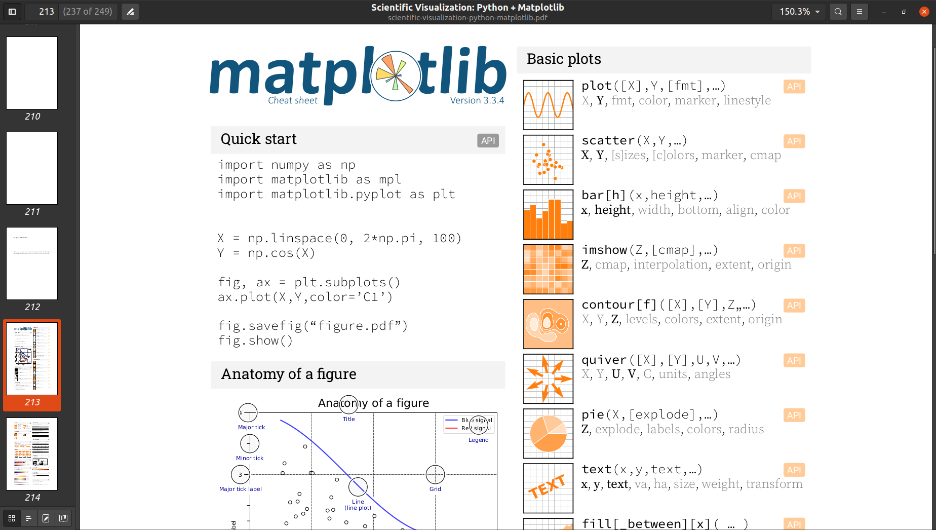
Fig. 25 matplotlib quick reference, from the Scientific Visualization: Python + Matplotlib book.

Note

The tutorials of matplotlib are also a good starting point to learn about the package. Scientific Visualization: Python + Matplotlib is a recommended book about advanced plotting methods using matplotlib (Fig. 25). It is can be downloaded as PDF.

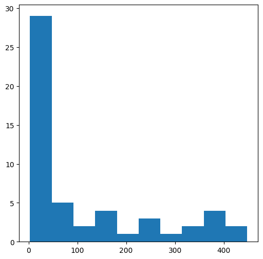
Histograms (numpy)

To make a histogram showing the distribution of a numpy array, we first need to “collect” them into one long on-dimensional array using the flatten method (see To one-dimensional (.flatten)):

v = m.flatten()
v

array([ nan,  nan,  nan,  nan,  nan,   3.,   3.,  nan,  nan,  nan,  nan,
         4.,   6.,   4.,  nan,  nan,  nan,  nan,   6.,   9.,   7.,  nan,
        61.,   9.,   4.,   9.,  10.,  16.,  nan, 106., 132.,  11.,   6.,
         6.,  27.,  nan,  47., 254., 146.,   6.,   6.,  12.,  nan,  31.,
       233., 340., 163.,  13.,  64.,   3.,  39., 253., 383., 448., 152.,
        39.,   5.,  32., 199., 357., 414., 360.,  48.,   7.,  49., 179.,
       307., 403., 370.,  55.])

Then, the one-dimensional array can be passed to the plt.hist function to produce a histogram:

plt.hist(v);

Note

The ; at the end of a matplotlib expression is an IPython trick to avoid printing textual data along with the plot. (Try removing it and re-running the cell to see the unwanted textual output.)

Line plots (numpy)

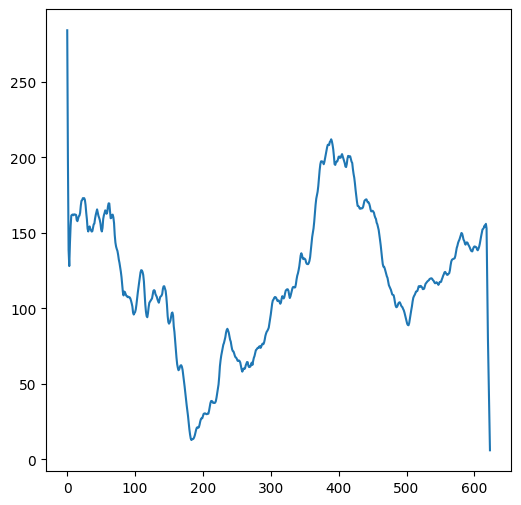
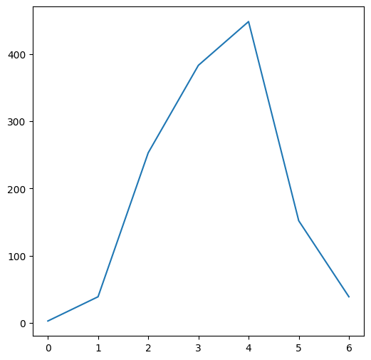
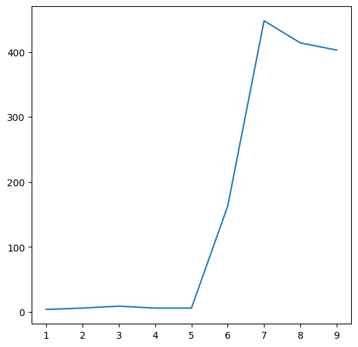
A one-dimensional array can be passed to the plt.plot function to display the array values in a line plot, where the x-axis values are array indices, and y-axis values are the array values. For example, the plt.plot can be used to display a “profile” or “slice” of a given array, along a specific row:

plt.plot(m[7, :]);

or along a specific column:

plt.plot(m[:, 4]);

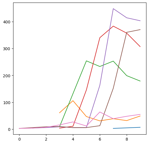
A two-dimensional array can also be passed to plt.plot, in which case each array column is plotted as a separate series. For example, the following plot displays the seven columns in m, i.e., seven north-south elevation profiles:

plt.plot(m);

Images (numpy)

To display the information of a two-dimensional array all at once, we can encode the array values into a visual property, such as color. The result is an image, also known as a heatmap. The plt.imshow (short for “image show”) function can be used to produce an image of a two-dimensional array:

plt.imshow(m);

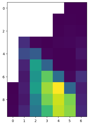
Since m is an array representing a Digital Elevation Model, this image is actually an elevation map of the area that this array represents.

Beyond numpy

numpy is a fundamental Python package, with many other packages for data analysis, scientific computing, and statistics depending on it. Notable packages depending on numpy include:

• pandas—For working with tables

• scipy—For scientific computations

• scikit-learn—For statistical analysis and machine learning

We are going to cover pandas in the next two chapters (see Tables (pandas) and Table reshaping and joins). Towards the end of the book we are going to breifly use scipy to apply a focal filter over a raster (see Focal filtering).

The scikit-learn package is beyond the scope of this book, however there are many resources online (https://scikit-learn.org/stable/) and in print. In case you are going to do statistical analysis or machine learning in Python, scikit-learn is the recommended starting point.

More exercises

Exercise 04-g

• Calculate a \(10\times 10\) array which contains the multiplication table (as shown below). Hint: create a “template” array of the right shape (with uniform values such as 0), then use a nested for loop (see for loops) to populate it with the correct values.

• Next, make your code general enough so that it can produce a multiplication table of any size, specified by a parameter named s in the beginning of the code. For example, s=10 should result in the \(10\times 10\) multiplication table shown below, s=5 should result in a \(5\times 5\) multiplication table, and so on.

array([[  1,   2,   3,   4,   5,   6,   7,   8,   9,  10],
       [  2,   4,   6,   8,  10,  12,  14,  16,  18,  20],
       [  3,   6,   9,  12,  15,  18,  21,  24,  27,  30],
       [  4,   8,  12,  16,  20,  24,  28,  32,  36,  40],
       [  5,  10,  15,  20,  25,  30,  35,  40,  45,  50],
       [  6,  12,  18,  24,  30,  36,  42,  48,  54,  60],
       [  7,  14,  21,  28,  35,  42,  49,  56,  63,  70],
       [  8,  16,  24,  32,  40,  48,  56,  64,  72,  80],
       [  9,  18,  27,  36,  45,  54,  63,  72,  81,  90],
       [ 10,  20,  30,  40,  50,  60,  70,  80,  90, 100]])

Exercise 04-h

• Read the 'carmel.csv' file into a numpy array (see Reading array from file).

• Find the minimum, maximum, and average elevation value in the Carmel area, according to the carmel.csv array, excluding “No Data” values (answer: -14.0, 541.0, and 124.06, respectively).

• Calculate and plot a new array where “No Data” values are flagged by 1, and any other value is flagged by 0 (Fig. 26).

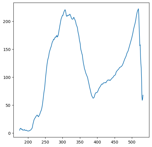
• Calculate the proportion of missing values in the array (answer: 0.53).

• Calculate and plot the average column and row “profiles” of the Carmel DEM, by calculating a 1D array of column means, and a 1D array of row means, respectively (Fig. 27).

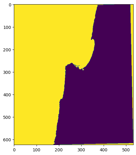
Fig. 26 Solution of exercise-04-h1: “No Data” values in carmel.csv

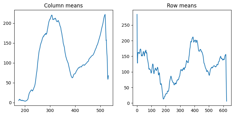
Fig. 27 Solution of exercise-04-h2: Column and row means of carmel.csv

Exercise solutions

Exercise 04-g

import numpy as np
# Shape (e.g., 10 for '10*10')
s = 10
# Create "template"
x = np.tile(0, s**2)
x = x.reshape((s, s))
# Calculate i*j
for i in np.arange(x.shape[0]):
    for j in np.arange(x.shape[1]):
        x[i,j] = (i+1)*(j+1)
# Print
x

array([[  1,   2,   3,   4,   5,   6,   7,   8,   9,  10],
       [  2,   4,   6,   8,  10,  12,  14,  16,  18,  20],
       [  3,   6,   9,  12,  15,  18,  21,  24,  27,  30],
       [  4,   8,  12,  16,  20,  24,  28,  32,  36,  40],
       [  5,  10,  15,  20,  25,  30,  35,  40,  45,  50],
       [  6,  12,  18,  24,  30,  36,  42,  48,  54,  60],
       [  7,  14,  21,  28,  35,  42,  49,  56,  63,  70],
       [  8,  16,  24,  32,  40,  48,  56,  64,  72,  80],
       [  9,  18,  27,  36,  45,  54,  63,  72,  81,  90],
       [ 10,  20,  30,  40,  50,  60,  70,  80,  90, 100]])

Exercise 04-h

import matplotlib.pyplot as plt
m = np.genfromtxt('data/carmel.csv', delimiter=',')
np.nanmin(m)

-14.0

np.nanmax(m)

541.0

m1 = np.isnan(m)
plt.imshow(m1);

m1.mean()

0.5275713186125944

colmeans = np.nanmean(m, axis=0)
rowmeans = np.nanmean(m, axis=1)

/tmp/ipykernel_21594/4262640268.py:1: RuntimeWarning: Mean of empty slice
  colmeans = np.nanmean(m, axis=0)

plt.plot(colmeans);

plt.plot(rowmeans);