Rasters (rasterio)

Last updated: 2024-03-05 11:28:38

---

Introduction

In this section we move on to the second type of spatial layers, rasters. Rasters are basically georeferenced images. That is, in additional to the numeric array that contains the image values, that every image has, a raster also has metadata specifying the rectangual extent that the image corresponds to in a particular spatial Coordinate Reference System. Rasters are stored in special formats, such as GeoTIFF ('.tif') or Erdas Imagine Image ('.img').

To work with rasters, we are going to use the rasterio package. The rasterio package is compatible with, and extends, the numpy package. Specifically, we will go over the following raster workflow:

• Reading raster files and examining their properties (see Raster file connection, Raster properties, and Reading raster data)

• Plotting rasters (see Plotting (rasterio))

• Creating a raster from a numpy array (see Creating raster from array)

• Writing raster to file (see Writing rasters)

• Making calculations with raster values (see “No Data” in rasters, and Working with raster values)

The rasterio package is not as comprehensive, and is lower level, compared to geopandas for vector layers. Therefore, many standard raster-related workflows are complicated to do with rasterio on its own. In the second part of this chapter and in the next one, we will demonstrate more specific tasks through additional third-party packages:

• richdem—for calculating topographic indices (see DEM calculations)

• scipy—for focal filtering (see Focal filtering)

• rasterstats—For zonal statistics of rasters (see Zonal statistics)

In the next chapter (see Raster-vector interactions), we are going to explore operations that involve both a raster and a vector layer, such as converting a raster to polygons, or extracting raster values to points or polygons.

Loading raster packages

In this chapter we use quite a few more packages than in any of the previous chapters. Let us go over the packages and their purpose, and load them, before we start working.

To start working with rasterio, first of all, we import the rasterio package, as well as the rasterio.plot sub-package (used for raster plotting):

import rasterio
import rasterio.plot

We will also load the numpy, shapely, and geopandas packages, which we use to load a numpy array and convert it to a raster (see Creating raster from array), for calculating the raster bounding box (see Raster extent), and loading a vector later for plotting (see Plotting a raster and a vector layer), respectively:

import numpy as np
import shapely
import geopandas as gpd

We load the glob standard package, which we breifly use to process multiple file paths when reading raster files (see Stacking raster bands):

import glob

We load matplotlib.pyplot (The matplotlib package) for plotting:

import matplotlib.pyplot as plt

Finally, we load richdem (see DEM calculations) and scipy.ndimage (see Focal filtering), which we use for specific raster processing tasks later on in this chapter:

import richdem as rd
import scipy.ndimage

What is rasterio?

rasterio is a third-party Python package for working with rasters. rasterio makes raster data accessible in the form of numpy arrays, so that we can operate on them, then write back to new raster files. rasterio, like most raster processing software, is based on the GDAL software. As mentioned above, working with rasters in Python is less well-organized around one comprehensive package (such as the case for vector layers and geopandas). Instead, there are several packages providing alternative (subsets of methods) of working with raster data.

The two most notable approaches for working with rasters in Python are provided by the rasterio (which we learn about in this chapter) and xarray packages. These two packages differ in their scope and underlying data models. Specifically, rasterio represents rasters as numpy arrays associated with a separate object holding the spatial metadata. The xarray package, however, represents rasters with the native DataArray object, which is an extension of numpy arrays designed to hold axis labels and attributes, in the same object, together with the array of raster values.

Both the rasterio and xarray packages are not comprehensive in the same way as geopandas is. For example, when working with rasterio, on the one hand, more packages may be needed to accomplish (commonly used) tasks such as zonal statistics (package rasterstats, see Zonal statistics) or calculating topographic indices (package richdem, see DEM calculations). On the other hand, xarray was extended to accommodate spatial operators missing from the core package itself, with the rioxarray and xarray-spatial packages.

Raster file connection

A raster data source, such as a GeoTIFF file, can be accessed using the rasterio.open function. This creates a connection to the raster data. The raster properties are imported instantly (see Raster properties). The raster data, however, are not automatically imported, as they are potentially very large and memory-consuming. Raster data can be read from the raster “connection” object created with rasterio.open in a separate step (see Reading raster data).

Note

Conceptually, a raster file connection object created with rasterio.open is similar to a text file connection object created with open (see File object and reading lines).

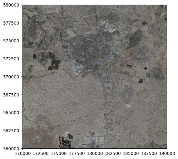
The BSV_res200-M.tif raster, provided with the sample data, is a three-band (red, green, blue) aerial photo of Beer-Sheva, taken at 2015, at 2 \(m\) resolution. The following expression creates a connection object named src to this raster:

src = rasterio.open('data/BSV_res200-M.tif')
src

<open DatasetReader name='data/BSV_res200-M.tif' mode='r'>

Note that the printout includes the mode='r' part, which indicates the dataset is opened in reading mode. This is the default mode of rasterio.open, so the following expression does exactly the same:

src = rasterio.open('data/BSV_res200-M.tif', 'r')
src

<open DatasetReader name='data/BSV_res200-M.tif' mode='r'>

Later on, we will see how a raster file can also be opened in writing mode ('w') when our intention is to write into a new raster file (see Writing rasters).

Raster properties

Overview

As mentioned above, the rasterio.open function creates a “connection” to a raster file, without reading the data, i.e., without actually reading the raster values. However, the essential file properties, or metadata, are being read and consequently contained in the file connection object (such as src). Let us go over these properties now.

The file name and connection mode can be obtained, from a raster file connection object, through its .name and .mode properties, respectively:

src.name

'data/BSV_res200-M.tif'

src.mode

'r'

Most of the other raster object properties can be accessed at once, through the .meta (“metadata”) property, which returns a dict as follows:

src.meta

{'driver': 'GTiff',
 'dtype': 'uint8',
 'nodata': None,
 'width': 10000,
 'height': 10000,
 'count': 3,
 'crs': None,
 'transform': Affine(2.0, 0.0, 170000.0,
        0.0, -2.0, 580000.0)}

There are also specific properties for direct access, as shown below.

Raster dimensions

The most fundamental property of a raster is its dimensions, namely, the number of layers, rows, and columns. These are stored in the following raster object properties:

• .count—Number of layers

• .height—Number of rows

• .width—Number of columns

For example, the raster BSV_res200-M.tif has three layers (corresponding to red, green, and blue channels), and 10,000 rows and columns:

src.count

3

src.height

10000

src.width

10000

Raster CRS

The raster Coordinate Reference System (CRS) is stored in the .crs property of the raster object, in the same format as we have seen for vector layers (see CRS and reprojection). The raster BSV_res200-M.tif does not contain a CRS definition, thus r.crs is equal to None and nothing is printed:

src.crs

Raster extent

Other than the CRS, for the raster to be geo-referenced we need to know the coordinates of the pixels. Since a raster is a regular rectangular grid, it is enough to know either one of the following:

• The origin and the resolution, i.e., the coordinates of one corner, typically the top-left (xmin, ymax) and the resolution (delta_x, delta_y)

• The bounding box, i.e., the coordinates of the bottom-left and the top-right corners (xmin, ymin, xmax, ymax), whereas the resolution can be determined according to the number of rows and columns

In rasterio, the extent information is given in the form of a transformation matrix, in the .transform property:

src.transform

Affine(2.0, 0.0, 170000.0,
       0.0, -2.0, 580000.0)

The values in the transform matrix provide the origin and resolution information, in the following form:

Affine(`delta_x`, 0.0, `xmin`,
       0.0, `delta_y`, `ymax`)

Notably, the x-axis and y-axis resolutions are identical, which is often the case, since raster pixels usually represent squares. The y-axis resolution is negative since, by convention, the origin is defined as the top-left corner (i.e., the y-axis origin is ymax and not ymin). Therefore, with each step along the raster rows we are actually going down rather than up, and y-axis values get progressively smaller.

The matrix can be multiplied by a pixel index, in the form (row,column), to obtain the coordinates of that point. For example, here are the coordinates of the top-left corner of the raster, i.e., row 0 and column 0:

src.transform * (0, 0)  ## Top-left raster corner

(170000.0, 580000.0)

Exercise 10-a

• Modify the above expression to find the coordinates of the bottom-right corner of the raster.

To get the center of the top-left pixel, we need to further move \(\frac {1}{2}\) of the resolution down and to the right, or use a fractional “index”:

src.transform * (0.5, 0.5)  ## Coordinates of top-left pixel center

(170001.0, 579999.0)

As we have just seen, the coordinates of the raster corners, i.e., its extent or bounds, can be derived from the .transform property and raster dimensions. However, the extent is also provided directly through the .bounds property:

src.bounds

BoundingBox(left=170000.0, bottom=560000.0, right=190000.0, top=580000.0)

The get one of the specific values we can further specify one of the internal properties, left, bottom, right, or top (corresponding to xmin, ymin, xmax, and ymax, respectively). For example:

src.bounds.left

170000.0

We can also convert the .bounds object to a shapely geometry using the shapely.box function (see Bounds (shapely)), as follows. This is very useful in case we need to evaluate the raster extent with respect to other layers, for example, to figure out whether an aerial photograph captures the entire area of a particular town.

shapely.box(*src.bounds)

Note that the expression uses the positional arguments technique (see Variable-length positional arguments).

Exercise 10-b

• How can we create a GeoDataFrame with one polygon feature, representing the raster bounds?

Plotting (rasterio)

Plotting a raster

To get a sense of the information in the raster, a basic plot can be produced using the rasterio.plot.show function. When the raster file connection contains three bands, these are treated as \(Red\), \(Green\), and \(Blue\) (in that order), and displayed as an RGB image:

rasterio.plot.show(src);

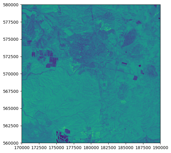
We can also pass a tuple with a raster file connection and an index of a particular band, in which case we get an image of that band only. Note that rasterio band numbering start from 1, so band 1 corresponds to the first (\(Red\)) band:

rasterio.plot.show((src, 1));

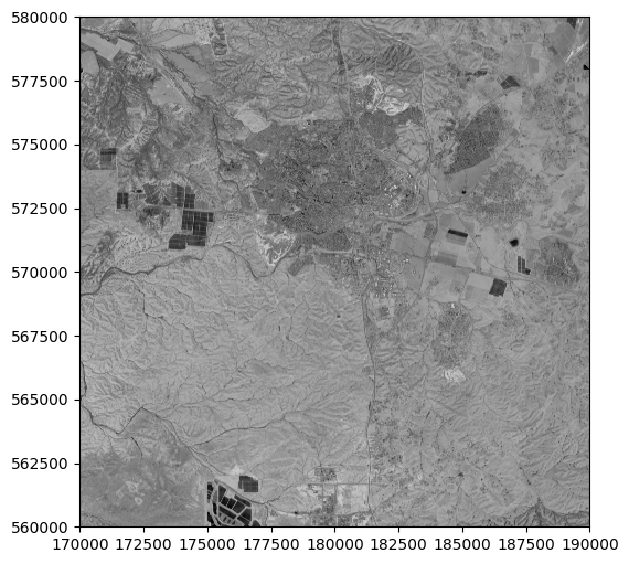
When displaying a single band, we can specify a color scale with the cmap argument, similarly to .plot in geopandas (see Setting symbology). It is standard practice to display a single band with the 'Greys_r' (“greys reversed”) color palette, where high values (i.e., high reflectance) appear bright, and low values appear dark:

rasterio.plot.show((src, 1), cmap='Greys_r');

Note

See Plotting in the rasterio documentation for more details and examples.

Plotting a raster and a vector layer

To plot a raster and a vector layers together, we need to initialize a plot object with plt.subplots, and pass the same ax argument to both plots. For example, let’s import the railway lines layer and filter the active lines (see Reading vector layers and Filtering by attributes):

rail = gpd.read_file('data/RAIL_STRATEGIC.shp')
rail = rail[rail['ISACTIVE'] == 'פעיל']

Here is how we can plot the railway lines and the aerial photo together:

fig, ax = plt.subplots()
rasterio.plot.show(src, ax=ax)
rail.plot(ax=ax, edgecolor='red');

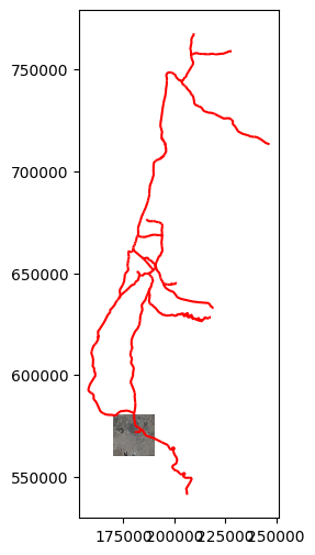
Keep in mind that, as usual, that both layers need to be in the same CRS for an operation involving both to make sense. In this case the BSV_res200-M.tif is in the ITM (EPSG 2039) CRS, same as RAIL_STRATEGIC.shp, even though the CRS definition is missing from the .tif file.

Reading raster data

Overview

As shown above, opening a raster file with rasterio.open creates a file connection object, containing raster metadata (see Raster file connection). However, the raster data, that is, the array of raster values, was not read into memory.

To read the raster values we need to use the .read method of the file connection object. The separation of creating a file connection and actually reading the raster values into separate steps may feel cumbersome. However, this type of design has advantages in terms of memory-use efficiency. For example, in case the raster is very large we can read only part of the information, or process it in consecutive “chunks”, so that we do not consume too much RAM which will make the computer “freeze”.

Reading all bands

To read all raster bands into an in-memory numpy array, we use the .read method without specifying any parameters. For example, the following expression reads the raster values from all bands, into an ndarray object named r:

r = src.read()
r

array([[[115, 132,  75, ..., 110, 103, 111],
        [133, 141, 135, ..., 105,  96,  94],
        [111, 147, 140, ...,  94,  97, 103],
        ...,
        [140,  68,  94, ..., 122, 128, 129],
        [148, 108, 124, ..., 131, 124, 134],
        [150, 119, 136, ..., 110, 137, 130]],

       [[111, 129,  75, ..., 101,  98, 106],
        [132, 140, 132, ...,  99,  92,  88],
        [111, 143, 136, ...,  87,  92,  96],
        ...,
        [133,  75,  89, ..., 120, 127, 127],
        [139, 105, 111, ..., 129, 126, 133],
        [140, 108, 128, ..., 104, 139, 127]],

       [[113, 122,  76, ...,  95,  90,  96],
        [125, 132, 128, ...,  90,  84,  83],
        [113, 137, 132, ...,  80,  84,  88],
        ...,
        [123,  74,  90, ..., 119, 121, 124],
        [128, 102, 104, ..., 124, 120, 127],
        [131, 106, 120, ..., 104, 134, 121]]], dtype=uint8)

Note

Thanks to the fact that numpy data types corresponds to file storage types, reading all raster values into memory consumes approximately the same amount of RAM as the file size on disk, that is, the minimal required amount of memory. For example, run the expression import sys; round(sys.getsizeof(r)/1024/1024,2) which returns the array object size, in Megabytes (MB), and compare the result with the original file size.

When reading all raster bands, we get a three-dimensional array. The order of the dimensions is (bands,rows,columns):

r.shape

(3, 10000, 10000)

Once we have an array with all bands, such as r, we can always subset a particular band (or any other type of subset), using the numpy subsetting methods (see Subsetting arrays). For example, the following expression “pulls out” a two-dimensional array with the values of the 1^st raster band:

r[0, :, :]

array([[115, 132,  75, ..., 110, 103, 111],
       [133, 141, 135, ..., 105,  96,  94],
       [111, 147, 140, ...,  94,  97, 103],
       ...,
       [140,  68,  94, ..., 122, 128, 129],
       [148, 108, 124, ..., 131, 124, 134],
       [150, 119, 136, ..., 110, 137, 130]], dtype=uint8)

We will also use the following shortcut, for clearer syntax of selecting an entire band, such as in raster algebra operations involving multiple bands (see Calculating indices):

r[0]

array([[115, 132,  75, ..., 110, 103, 111],
       [133, 141, 135, ..., 105,  96,  94],
       [111, 147, 140, ...,  94,  97, 103],
       ...,
       [140,  68,  94, ..., 122, 128, 129],
       [148, 108, 124, ..., 131, 124, 134],
       [150, 119, 136, ..., 110, 137, 130]], dtype=uint8)

Reading specific bands

In case we need specific bands, to conserve memory, it is better to read just the band we need in the first place. This can be done by specifying the band index inside .read. Keep in mind that rasterio band indices starts from 1. For example, here we read each of the bands 1, 2, and 3, into separate arrays named red, green, and blue, respectively:

red = src.read(1)
green = src.read(2)
blue = src.read(3)

Each of red, green, and blue is a two-dimensional array. For example:

red.shape

(10000, 10000)

Again, note that .read() imports the raster data into a three-dimensional array, while .read(1), .read(2), etc. import the raster data into a two-dimensional array. Therefore, .read() and .read(1) do not produce the same result even if the raster data source is one-dimensional. Here is a short demonstration, using a single-band raster file which we will work with later on (see Stacking raster bands):

rasterio.open('data/T36RXV_20201226T082249_B02.jp2').read().shape

(1, 2968, 3554)

rasterio.open('data/T36RXV_20201226T082249_B02.jp2').read(1).shape

(2968, 3554)

It is also possible to read several bands at once, by specifying a list of bands. For example, here we read the third and second bands (in that order):

src.read([3, 2])

array([[[113, 122,  76, ...,  95,  90,  96],
        [125, 132, 128, ...,  90,  84,  83],
        [113, 137, 132, ...,  80,  84,  88],
        ...,
        [123,  74,  90, ..., 119, 121, 124],
        [128, 102, 104, ..., 124, 120, 127],
        [131, 106, 120, ..., 104, 134, 121]],

       [[111, 129,  75, ..., 101,  98, 106],
        [132, 140, 132, ...,  99,  92,  88],
        [111, 143, 136, ...,  87,  92,  96],
        ...,
        [133,  75,  89, ..., 120, 127, 127],
        [139, 105, 111, ..., 129, 126, 133],
        [140, 108, 128, ..., 104, 139, 127]]], dtype=uint8)

Creating raster from array

In some cases, we may need to go the other way around: transforming an array into a raster. For example, we may be given an array (e.g., in a CSV file) and the extent and CRS information, and asked to store the information in a spatial raster file format such as GeoTIFF. As we have seen above, a raster is just an array associated with spatial metadata, namely:

• Origin and resolution (.transform)

• CRS definition (.crs)

Therefore, going from an array to a raster technically means we need to construct the .transform and .crs objects.

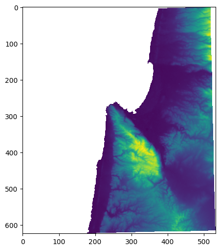
To demonstrate, let’s import the 'carmel.csv' matrix, which contains a Digital Elevation Model (DEM) of the area around Haifa (see Reading array from file):

m = np.genfromtxt('data/carmel.csv', delimiter=',')
m

array([[nan, nan, nan, ..., nan, nan, nan],
       [nan, nan, nan, ..., nan, nan, nan],
       [nan, nan, nan, ..., nan, nan, nan],
       ...,
       [nan, nan, nan, ..., nan, nan, nan],
       [nan, nan, nan, ..., nan, nan, nan],
       [nan, nan, nan, ..., nan, nan, nan]])

Using the rasterio.plot.show function, here is a visualization of the resulting m array:

rasterio.plot.show(m);

The m array is defined as float64:

m.dtype

dtype('float64')

However, it actually contains only integers. To be more efficient, we will therefore convert (see Changing data type) it to an int16 array. Since int arrays cannot contain “No Data” values (see “No Data” representation), we are going to encode “No Data” as -9999, which is a value never encountered in DEMs and a common convention:

m[np.isnan(m)] = -9999
m = m.astype(np.int16)
m

array([[-9999, -9999, -9999, ..., -9999, -9999, -9999],
       [-9999, -9999, -9999, ..., -9999, -9999, -9999],
       [-9999, -9999, -9999, ..., -9999, -9999, -9999],
       ...,
       [-9999, -9999, -9999, ..., -9999, -9999, -9999],
       [-9999, -9999, -9999, ..., -9999, -9999, -9999],
       [-9999, -9999, -9999, ..., -9999, -9999, -9999]], dtype=int16)

Why is -9999 a good choice for representing “No Data” values in a DEM?

• It is invalid with repect to the measured variable, since there is no place on earth where elevation is -9999 meters below sea level. If someone encounters the value -9999 in a DEM, they can be fairly certain that it represents “No Data” even without looking into the metadata.

• It is extreme. Therefore, if it accidently does get into a calculation (such as zonal mean of elevation), there is a good chance the results are going to be skewed which will catch the analysts’ attention so that they can spot the mistake.

Now, what’s missing is the raster georeferencing information: the .transform matrix and the CRS definition. This information needs to be known in advance. If we do not have it, we can try to manually georeference the raster using control points (such as landmarks, trees, large stones, etc.), however this may be difficult and error-prone, unless the raster is a high-resolution aerial photograph. In this example, let us assume that the origin and resolution of the raster are known in advance. In such case, we can use the rasterio.transform.from_origin function to create a .transform object:

new_transform = rasterio.transform.from_origin(
    west=662317, 
    north=3658412, 
    xsize=90, 
    ysize=90
)
new_transform

Affine(90.0, 0.0, 662317.0,
       0.0, -90.0, 3658412.0)

Also, let’s assume that we know the CRS of the raster, and that it is UTM Zone 36N (32636).

Now we have all necessary information to export the Haifa DEM into a spatial raster format such as GeoTIFF, which is what we do next.

Writing rasters

Writing single-band (int)

To write an array into a raster file, we need to pass a (non-existing) raster file path to rasterio.open, in writing ('w') mode. As opposed to read mode, the rasterio.open function needs quite a lot of information (in addition to the file path and mode):

• driver—The file format (The recommendation is 'GTiff')

• height—Number of rows

• width—Number of columns

• count—Number of bands

• nodata—The value which represents “No Data”, if any

• dtype—The raster data type, one of numpy types supported by the driver (e.g., np.int16)

• crs—The CRS, using an EPSG code (e.g., 32636)

• transform—The transform matrix

• compress—a compression method to apply, such as 'lzw'. This is optional and most useful for large rasters. Note that, at the time of writing, this doesn’t work well for writing multiband rasters.

Note

Note that 'GTiff (GeoTIFF, .tif), which is the recommended driver, supports just some of the possible numpy data types (Table 12; also see GDAL documentation). Importantly, it does not support np.int64, the default int type. The recommendation in such case it to use np.int32 (if the range is sufficient), or np.float64.

We already have all the necessary information. Here is the expression to open a GeoTIFF file named 'carmel.tif' in writing mode, with the right arguments to store the Haifa DEM values in array m:

new_dataset = rasterio.open(
    'output/carmel.tif', 'w', 
    driver = 'GTiff',
    height = m.shape[0],
    width = m.shape[1],
    count = 1,
    nodata = -9999,
    dtype = m.dtype,
    crs = 32636,
    transform = new_transform,
    compress='lzw'
)

Exercise 10-c

• Go over the arguments in the above rasterio.open function call, and make sure you understand where they come from and what is their meaning.

Note that the data are not written into the file yet! To do that, once the file connection is ready, we use the .write method to actually write the array into the file connection. When writing, we need to specify the array with the data to write (such as m), and the band index where the data will be written. Note that the band index starts from 1:

new_dataset.write(m, 1)

In the end, we must “close” the file connection using the .close method. This is particularly important in writing mode, as closing assures that writing is completed:

new_dataset.close()

Writing single-band (float)

In case we choose to write a float raster, the recommendation is to specify missing values using np.nan. To demonstrate, let us go back to the original float64 array:

m = np.genfromtxt('data/carmel.csv', delimiter=',')
m

array([[nan, nan, nan, ..., nan, nan, nan],
       [nan, nan, nan, ..., nan, nan, nan],
       [nan, nan, nan, ..., nan, nan, nan],
       ...,
       [nan, nan, nan, ..., nan, nan, nan],
       [nan, nan, nan, ..., nan, nan, nan],
       [nan, nan, nan, ..., nan, nan, nan]])

The following expressions writing the array into another file named 'carmel2.tif'. The arguments in rasterio.open are almost identical, except for nodata which is left unspecified:

new_dataset = rasterio.open(
    'output/carmel2.tif', 'w', 
    driver = 'GTiff',
    height = m.shape[0],
    width = m.shape[1],
    count = 1,
    dtype = m.dtype,
    crs = 32636,
    transform = new_transform
)
new_dataset.write(m, 1)
new_dataset.close()

The resulting raster is going to have a “native” encoding of “No Data”, with no need to specify a particular numeric value such as -9999. When reading the raster back into an array, the “No Data” will be interpreted as np.nan:

rasterio.open('output/carmel2.tif').read()

array([[[nan, nan, nan, ..., nan, nan, nan],
        [nan, nan, nan, ..., nan, nan, nan],
        [nan, nan, nan, ..., nan, nan, nan],
        ...,
        [nan, nan, nan, ..., nan, nan, nan],
        [nan, nan, nan, ..., nan, nan, nan],
        [nan, nan, nan, ..., nan, nan, nan]]])

Stacking raster bands

Remote sensing products, such as satellite images, are often distributed as a collection of single-band files, one file for each spectral band of the sensor. For example, Landsat and Sentinel satellite images are distributed in this way. In this section, we are going to learn how to “stack” separate single-band raster files into a multi-band raster which is easier to work with, and to view in GIS software.

First, we will create a list with the file paths of the separate raster files which we are going to stack. The sample image is a Sentinel-2 satellite image of central/southern Israel from 2020-12-26. Sentinel-2 satellite images are distributed in a raster format called JPEG2000 (.jp2). The image original contains 14 bands. To keep things more simple, the sample data contains just four out of 14 files, the ones which are usually important: the red, green, blue, and Near Infrared bands. Here are their file paths:

pattern = 'data/T36RXV_20201226T082249_'
files = [
    pattern + 'B02.jp2',  # Blue
    pattern + 'B03.jp2',  # Green
    pattern + 'B04.jp2',  # Red
    pattern + 'B08.jp2'   # NIR
]
files

['data/T36RXV_20201226T082249_B02.jp2',
 'data/T36RXV_20201226T082249_B03.jp2',
 'data/T36RXV_20201226T082249_B04.jp2',
 'data/T36RXV_20201226T082249_B08.jp2']

The above code section requires that we manually type the file name components, and that we know in advance the number of files. A more automated approach would be to search the files according to a patrticular pattern inside a given directory. For example, relying on the fact that the Sentinel-2 images files we are interested in are located in the data directory and characterized by the .jp2 extension, we can get the same list with their paths using shorter code, and the taking advantage of the glob standard package, as follows:

files = glob.glob('data/*.jp2')
files

['data/T36RXV_20201226T082249_B08.jp2',
 'data/T36RXV_20201226T082249_B02.jp2',
 'data/T36RXV_20201226T082249_B03.jp2',
 'data/T36RXV_20201226T082249_B04.jp2']

However, in this case we also need to manually sort (see list methods) the files, so that they match the intended order of bands in the multi-band raster we will be writing:

files.sort()
files

['data/T36RXV_20201226T082249_B02.jp2',
 'data/T36RXV_20201226T082249_B03.jp2',
 'data/T36RXV_20201226T082249_B04.jp2',
 'data/T36RXV_20201226T082249_B08.jp2']

Since the files comprise “bands” of the same image, the spatial metadata of all images is identical. Therefore, to write a multi-band raster we are going to use the spatial metadata from one of the images. It does not matter which one, so we are going to use the first image. First, we create the file connection:

src = rasterio.open(files[0])
src

<open DatasetReader name='data/T36RXV_20201226T082249_B02.jp2' mode='r'>

Then, we extract the spatial metadata (see Raster properties), and keep it in a separate object which we will use later on:

meta = src.meta
meta

{'driver': 'JP2OpenJPEG',
 'dtype': 'uint16',
 'nodata': None,
 'width': 3554,
 'height': 2968,
 'count': 1,
 'crs': CRS.from_epsg(32636),
 'transform': Affine(10.000856049521643, 0.0, 652642.4115,
        0.0, -10.000219878706249, 3473256.1222)}

Before we can use this meta object when writing the multi-band raster, we need to modify two of its properties:

• count—The number of bands, needs to be 4 instead of 1

• driver—Needs to be GeoTIFF ('GTiff') instead of JPEG2000, since this is the file format is best supported for writing with rasterio (see Writing single-band (int))

rasterio has a specialized method named .update, to update metadata objects, as follows:

meta.update(count=len(files))
meta.update(driver='GTiff')

Let us check the meta object to make sure the properties were actually updated:

meta

{'driver': 'GTiff',
 'dtype': 'uint16',
 'nodata': None,
 'width': 3554,
 'height': 2968,
 'count': 4,
 'crs': CRS.from_epsg(32636),
 'transform': Affine(10.000856049521643, 0.0, 652642.4115,
        0.0, -10.000219878706249, 3473256.1222)}

Now that we have the list of files (files), and the updated spatial metadata from one of the files (meta), we proceed to actually writing the multi-band raster. Here is the code to do that:

dst = rasterio.open('output/sentinel2.tif', 'w', **meta)
for index, filename in enumerate(files, start=1):
    src = rasterio.open(filename)
    dst.write(src.read(1), index)
    src.close()
dst.close()

This code section is relatively complex, so we will now go over the main points to pay attention to. First, note that we have two rasterio.open expressions:

• On the “top” level, we open a file named 'output/sentinel2.tif' (which may not exist yet) in writing mode as dst. This is where we write the multi-band raster. Note that we pass the meta object as keyword arguments (see Variable-length keyword arguments) with **meta.

• Inside the for loop which goes over the files, we open each file in reading mode. Using the enumerate technique (see Using enumerate), in each iteration we have access to the current band index starting from 1 (i.e., 1, 2, 3, and 4) and the current file name (filename). Inside the loop, we then read the first (and only) band of each file (src.read), and immediately write it to the respective band index in the destination file (dst.write(..., index)).

The above code created a new file named 'sentinel2.tif', which we can now read back into the Python session to work with it:

src = rasterio.open('output/sentinel2.tif')
src

<open DatasetReader name='output/sentinel2.tif' mode='r'>

Examining the metadata tells us that this is indeed a four-band raster:

src.meta

{'driver': 'GTiff',
 'dtype': 'uint16',
 'nodata': None,
 'width': 3554,
 'height': 2968,
 'count': 4,
 'crs': CRS.from_epsg(32636),
 'transform': Affine(10.000856049521643, 0.0, 652642.4115,
        0.0, -10.000219878706249, 3473256.1222)}

Here is how we can read all layers at once into a three-dimensional array named r:

r = src.read()
r

array([[[1600, 1560, 1598, ..., 1272, 1315, 1316],
        [1614, 1570, 1608, ..., 1196, 1262, 1316],
        [1630, 1584, 1619, ..., 1131, 1191, 1295],
        ...,
        [1597, 1576, 1599, ..., 2149, 2201, 2169],
        [1602, 1597, 1569, ..., 2220, 2237, 2228],
        [1577, 1577, 1563, ..., 2191, 2296, 2195]],

       [[1735, 1681, 1719, ..., 1361, 1396, 1358],
        [1747, 1711, 1723, ..., 1245, 1356, 1398],
        [1766, 1754, 1739, ..., 1133, 1240, 1344],
        ...,
        [1738, 1722, 1747, ..., 2501, 2602, 2647],
        [1736, 1736, 1705, ..., 2655, 2684, 2671],
        [1688, 1690, 1680, ..., 2652, 2719, 2693]],

       [[2107, 2101, 2107, ..., 1514, 1610, 1568],
        [2120, 2108, 2104, ..., 1294, 1510, 1549],
        [2140, 2124, 2109, ...,  983, 1248, 1463],
        ...,
        [2224, 2229, 2250, ..., 3265, 3337, 3440],
        [2248, 2195, 2229, ..., 3486, 3468, 3556],
        [2207, 2163, 2229, ..., 3452, 3574, 3529]],

       [[2793, 2710, 2797, ..., 2810, 2750, 2727],
        [2871, 2759, 2770, ..., 2930, 2908, 2821],
        [2859, 2793, 2807, ..., 2995, 2969, 2888],
        ...,
        [2682, 2720, 2733, ..., 3649, 3774, 3802],
        [2707, 2671, 2668, ..., 3851, 3905, 3919],
        [2639, 2624, 2665, ..., 3816, 4025, 3892]]], dtype=uint16)

When plotting an RGB image of the raster we need to make sure the bands are arranged in the Red-Green-Blue order, as follows. Nevertheless, something goes wrong and we see a balnk image. The problem is that (as stated in the printed message) integer values are interpreted as occupying the 0-255 range, while in this case the values are reflectance (0-1) multiplied by 10000, thus occupything the 0-10000 range. We are going to fix this shortly (see Rescaling).

rasterio.plot.show(r[[2, 1, 0], :, :]);

Clipping input data to the valid range for imshow with RGB data ([0..1] for floats or [0..255] for integers).

“No Data” in rasters

Overview

Rasters may contain “No Data”, i.e., pixels that have missing values. For example, remote sensing data, such as satellite images, may contain “No Data” pixel values to mark unreliable or unusable values, due to atmospheric interference such as clouds. In other cases, the “No Data” values may be used to mask the pixels beyond the area of interest, such as elevation over water bodies (see Writing rasters).

“No Data” representation (int)

An int raster file that has “No Data” must store a flag that specified which specific value is used to represent “No Data”, accessible through the .nodata property (see Raster properties).

As discussed earlier, due to memory-related limitations (see “No Data” representation), missing values cannot be represented by np.nan in int arrays. Accordingly, when reading an int raster into an array, .nodata values are interpreted as ordinary numeric values (such as -9999). It is up to the user to decide what to do in such case:

• Keep the raster as is, while being mindful of the numeric value representing “No Data” and excluding them from calculations

• Use a “No Data” mask along with the raster values (see “No Data” masks)

• Transforming the raster to float, then replace “No Data” values with np.nan

“No Data” representation (float)

A float raster that has “No Data” may, or may not, specify a particular numeric value as .nodata, since it can also use the native “No Data” value which does not require specifying one. Therefore, confusingly, float rasters can represent “No Data” values using either of two approaches:

• A “native”, data type-specific, encoding, in which case the “No Data” values are automatically interpreted as np.nan

• A specific numeric value, such as -9999, in which case the value is being interpreted as is (i.e., as -9999) similarly to int (see “No Data” representation (int))

Here is an example of the first case (see Writing single-band (float)), native “No Data” encoding which is automatically translated to np.nan:

rasterio.open('output/carmel2.tif').meta

{'driver': 'GTiff',
 'dtype': 'float64',
 'nodata': None,
 'width': 533,
 'height': 624,
 'count': 1,
 'crs': CRS.from_epsg(32636),
 'transform': Affine(90.0, 0.0, 662317.0,
        0.0, -90.0, 3658412.0)}

rasterio.open('output/carmel2.tif').read()

array([[[nan, nan, nan, ..., nan, nan, nan],
        [nan, nan, nan, ..., nan, nan, nan],
        [nan, nan, nan, ..., nan, nan, nan],
        ...,
        [nan, nan, nan, ..., nan, nan, nan],
        [nan, nan, nan, ..., nan, nan, nan],
        [nan, nan, nan, ..., nan, nan, nan]]])

Here is an example of the second case (Topographic aspect), “No Data” encoded using a numeric value which is not translated to np.nan:

rasterio.open('output/carmel_aspect.tif').meta

{'driver': 'GTiff',
 'dtype': 'float32',
 'nodata': -9999.0,
 'width': 533,
 'height': 624,
 'count': 1,
 'crs': CRS.from_epsg(32636),
 'transform': Affine(90.0, 0.0, 662317.0,
        0.0, -90.0, 3658412.0)}

rasterio.open('output/carmel_aspect.tif').read()

array([[[-9999., -9999., -9999., ..., -9999., -9999., -9999.],
        [-9999., -9999., -9999., ..., -9999., -9999., -9999.],
        [-9999., -9999., -9999., ..., -9999., -9999., -9999.],
        ...,
        [-9999., -9999., -9999., ..., -9999., -9999., -9999.],
        [-9999., -9999., -9999., ..., -9999., -9999., -9999.],
        [-9999., -9999., -9999., ..., -9999., -9999., -9999.]]],
      dtype=float32)

The latter behavior may seem inconvenient. However, it makes sure that treatment of the .nodata flag is the same in both int and float rasters.

“No Data” masks

Let us go back to the 'carmel.tif' raster with the DEM of the Carmel area created earlier (see Writing rasters). Recall that the numpy array with raster values which we wrote to file contained missing values (in the form of np.nan), representing undetermined elevation for the Mediterranean sea. Before writing it to the 'carmel.tif' raster file, we chose to convert the values into int, which, due to computer memory limitations, cannot represent np.nan. Therefore np.nan values were encoded as -9999, and the nodata=-9999 flag was specified in the 'carmel.tif' file metadata (see Writing rasters).

Indeed, if we read back the file 'carmel.tif', we can see that the .nodata property is set to -9999 in the raster metadata:

src = rasterio.open('output/carmel.tif')
src.meta

{'driver': 'GTiff',
 'dtype': 'int16',
 'nodata': -9999.0,
 'width': 533,
 'height': 624,
 'count': 1,
 'crs': CRS.from_epsg(32636),
 'transform': Affine(90.0, 0.0, 662317.0,
        0.0, -90.0, 3658412.0)}

As discussed above, when reading the data using .read (whether int or float), the values .nodata values are read as is:

src.read(1)

array([[-9999, -9999, -9999, ..., -9999, -9999, -9999],
       [-9999, -9999, -9999, ..., -9999, -9999, -9999],
       [-9999, -9999, -9999, ..., -9999, -9999, -9999],
       ...,
       [-9999, -9999, -9999, ..., -9999, -9999, -9999],
       [-9999, -9999, -9999, ..., -9999, -9999, -9999],
       [-9999, -9999, -9999, ..., -9999, -9999, -9999]], dtype=int16)

What can we do in case when a raster encodes “No Data” as a specific numeric value, and yet we would like to ignore that value in calculations? One of the the solutions is to use a “No Data” mask, i.e., an additional array which indicates which values in the original array are valid, or “No Data”.

There are two ways to create a “No Data” mask with rasterio. First, using the additional masked=True argument of .read, we can read the raster data into a special type of a numpy array known as a masked array:

r = src.read(1, masked=True)
r

masked_array(
  data=[[--, --, --, ..., --, --, --],
        [--, --, --, ..., --, --, --],
        [--, --, --, ..., --, --, --],
        ...,
        [--, --, --, ..., --, --, --],
        [--, --, --, ..., --, --, --],
        [--, --, --, ..., --, --, --]],
  mask=[[ True,  True,  True, ...,  True,  True,  True],
        [ True,  True,  True, ...,  True,  True,  True],
        [ True,  True,  True, ...,  True,  True,  True],
        ...,
        [ True,  True,  True, ...,  True,  True,  True],
        [ True,  True,  True, ...,  True,  True,  True],
        [ True,  True,  True, ...,  True,  True,  True]],
  fill_value=-9999,
  dtype=int16)

Detailed description of the masked array data structure is beyond the scope of this book. In short, a masked array is composed of two components:

• .data—The data (e.g., dem1.data)

• .mask—A boolean “NoData” mask (e.g., dem1.mask)

For example:

r.data

array([[-9999, -9999, -9999, ..., -9999, -9999, -9999],
       [-9999, -9999, -9999, ..., -9999, -9999, -9999],
       [-9999, -9999, -9999, ..., -9999, -9999, -9999],
       ...,
       [-9999, -9999, -9999, ..., -9999, -9999, -9999],
       [-9999, -9999, -9999, ..., -9999, -9999, -9999],
       [-9999, -9999, -9999, ..., -9999, -9999, -9999]], dtype=int16)

r.mask

array([[ True,  True,  True, ...,  True,  True,  True],
       [ True,  True,  True, ...,  True,  True,  True],
       [ True,  True,  True, ...,  True,  True,  True],
       ...,
       [ True,  True,  True, ...,  True,  True,  True],
       [ True,  True,  True, ...,  True,  True,  True],
       [ True,  True,  True, ...,  True,  True,  True]])

Importantly, numpy operators and functions are aware of the “No Data” mask, and automatically exclude the masked values from calculations. For example:

r.mean()

124.0609638124817

Second, we can read the data as an ordinary array using plain .read, and then also read the “No Data” mask into a separate array using the .read_masks method:

r = src.read(1)
mask = src.read_masks(1)

In the resulting “NoData” array, missing values are indicated by 0, while valid values are indicated by 255:

mask

array([[0, 0, 0, ..., 0, 0, 0],
       [0, 0, 0, ..., 0, 0, 0],
       [0, 0, 0, ..., 0, 0, 0],
       ...,
       [0, 0, 0, ..., 0, 0, 0],
       [0, 0, 0, ..., 0, 0, 0],
       [0, 0, 0, ..., 0, 0, 0]], dtype=uint8)

In this case, it is up to the user to exclude the masked values where necessary.

Working with raster values

Overview

Now that we know how to gain access to raster data, in the form of numpy arrays, we can perform many types of common raster operations which require just the raster values. For exampe:

• Summarizing values—Summarize raster values, globally or separately per band

• Rescaling—Linearly translate the raster values to a different data range

• Calculating indices—Calculating a single-band raster using a formula, applied on several raster bands, such as calculating an NDVI image from red and near-infrared bands

• Reclassifying—Convert a continuous raster to a categorical one

We will now see an example of each.

Summarizing values

For the next examples, let,s go back to the Sentinel-2 image:

src = rasterio.open('output/sentinel2.tif')
r = src.read()

To summarize raster values, either globally, or for specific dimensions, we can use numpy functions, possibly specifying the axis argument (see Global summaries). For example, the “global” minimum and maximum values of the raster—across the all bands and pixels—can be obtained with:

np.min(r)

0

np.max(r)

27999

To get the minimum and maximum of all pixels separately per band, recall that rasterio places the bands into the 0 dimension:

r.shape

(4, 2968, 3554)

Therefore, we need to specify axis=(1,2), i.e., the axes that we want to summarize and “discard” are 1 and 2 (see Summaries per dimension (3D)). For example, here are the minimum values in each of the four bands of the Sentinel-2 image:

np.min(r, axis=(1, 2))

array([ 94,   0,   0, 284], dtype=uint16)

and here are the maximum values:

np.max(r, axis=(1, 2))

array([27994, 26490, 27992, 27999], dtype=uint16)

Exercise 10-d

• Write an expression that returns the average value per pixel.

• The result should be a two-dimensional array of size 2968*3554 (check your answer using the .shape property).

Rescaling

Rescaling and calculating indices (see Calculating indices) are examples of operations that are applied on each pixel, separately, to compose a new raster with the results. This type of operations are collectively known as raster algebra.

For example, the Sentinel-2 images are stored as uint16, for conserving storage space, but they need to be rescaled by dividing each pixel value by 10000 to get the true reflectance values. This is a common “compression” technique when storing satellite images.

To get the reflectance values, we need to rescale all values dividing the entire array by 10000:

r = r / 10000
r

array([[[0.16  , 0.156 , 0.1598, ..., 0.1272, 0.1315, 0.1316],
        [0.1614, 0.157 , 0.1608, ..., 0.1196, 0.1262, 0.1316],
        [0.163 , 0.1584, 0.1619, ..., 0.1131, 0.1191, 0.1295],
        ...,
        [0.1597, 0.1576, 0.1599, ..., 0.2149, 0.2201, 0.2169],
        [0.1602, 0.1597, 0.1569, ..., 0.222 , 0.2237, 0.2228],
        [0.1577, 0.1577, 0.1563, ..., 0.2191, 0.2296, 0.2195]],

       [[0.1735, 0.1681, 0.1719, ..., 0.1361, 0.1396, 0.1358],
        [0.1747, 0.1711, 0.1723, ..., 0.1245, 0.1356, 0.1398],
        [0.1766, 0.1754, 0.1739, ..., 0.1133, 0.124 , 0.1344],
        ...,
        [0.1738, 0.1722, 0.1747, ..., 0.2501, 0.2602, 0.2647],
        [0.1736, 0.1736, 0.1705, ..., 0.2655, 0.2684, 0.2671],
        [0.1688, 0.169 , 0.168 , ..., 0.2652, 0.2719, 0.2693]],

       [[0.2107, 0.2101, 0.2107, ..., 0.1514, 0.161 , 0.1568],
        [0.212 , 0.2108, 0.2104, ..., 0.1294, 0.151 , 0.1549],
        [0.214 , 0.2124, 0.2109, ..., 0.0983, 0.1248, 0.1463],
        ...,
        [0.2224, 0.2229, 0.225 , ..., 0.3265, 0.3337, 0.344 ],
        [0.2248, 0.2195, 0.2229, ..., 0.3486, 0.3468, 0.3556],
        [0.2207, 0.2163, 0.2229, ..., 0.3452, 0.3574, 0.3529]],

       [[0.2793, 0.271 , 0.2797, ..., 0.281 , 0.275 , 0.2727],
        [0.2871, 0.2759, 0.277 , ..., 0.293 , 0.2908, 0.2821],
        [0.2859, 0.2793, 0.2807, ..., 0.2995, 0.2969, 0.2888],
        ...,
        [0.2682, 0.272 , 0.2733, ..., 0.3649, 0.3774, 0.3802],
        [0.2707, 0.2671, 0.2668, ..., 0.3851, 0.3905, 0.3919],
        [0.2639, 0.2624, 0.2665, ..., 0.3816, 0.4025, 0.3892]]])

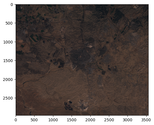
Now that we have a float64 raster with values between 0 and 1, we can observe an RGB image of the raster as follows:

rasterio.plot.show(r[[2, 1, 0], :, :]);

Clipping input data to the valid range for imshow with RGB data ([0..1] for floats or [0..255] for integers).

Reclassifying

When examining the range of values, we find out that we have values above 1, even though valid values of reflectance are between 0 and 1:

[r.min(), r.max()]

[0.0, 2.7999]

Exercise 10-e

• How many values >1 do we have in a? (answer: 228)

• How many pixels with at least one value >1 do we have? (answer: 120)

Higher values can arise, for example, as an interaction between particular atmospheric correction algorithms and particular surface characteristics. These values are considered outliers and usually are either replace with 1 or transformed to “No Data”.

This is an example of reclassifying, grouping all or same ranges of data values in the raster into uniform categories where all pixels share the same value. In this case, we want to replace all pixels with >1 into 1. Technically, this is a numpy “assignment to subset” operation, which we are already familiar with (see Masking):

r[r > 1] = 1

Let us check the data range of the modified raster. Indeed, the data range is now 0-1:

[r.min(), r.max()]

[0.0, 1.0]

Calculating indices

Calculating indices is a raster algebra operation where we use a particular formula to calculate a single-band image, from a multi-band image. The formula is applied on the values of each pixel, separately, and the individual calculations then comprise the resulting single-band image. There is a wide variety of useful indices developed in image analysis and remote sensing practice. We will see two examples:

• Calculating a greyscale image from red, green, and blue bands

• Calculating an NDVI image from red and near-infrared bands

Let’s start with the grayscale image. Given \(Red\), \(Green\), and \(Blue\), bands, a simple formula for a greyscale image is calculating the weighted average reflectance from all three bands, as follows:

\[Grey=0.2125 \times Red + 0.7154 \times Green + 0.0721 \times Blue\]

In the resulting greyscale image, pixels that have high averaged reflectance will have high greyscale values and will appear bright. Pixels that have low average reflectance will appear dark.

Here is how we can calculate a greyscale image from our Sentinel-2 data, using numpy vectorized arithmetic operations (see Vectorized operations):

greyscale = 0.2125*r[2] + 0.7154*r[1] + 0.0721*r[0]
greyscale

array([[0.18043165, 0.17615259, 0.17927259, ..., 0.13870956, 0.14356349,
        0.13995968],
       [0.18166732, 0.17851964, 0.1795671 , ..., 0.12518796, 0.13819476,
        0.14241753],
       [0.18356694, 0.1820368 , 0.1808973 , ..., 0.11009808, 0.12381671,
        0.13657546],
       ...,
       [0.18311089, 0.18192109, 0.18432167, ..., 0.26379708, 0.27292754,
        0.27810487],
       [0.18351386, 0.18235156, 0.18065444, ..., 0.2800224 , 0.28183713,
        0.28271222],
       [0.17902844, 0.17823652, 0.17882268, ..., 0.27887619, 0.28701892,
        0.28347442]])

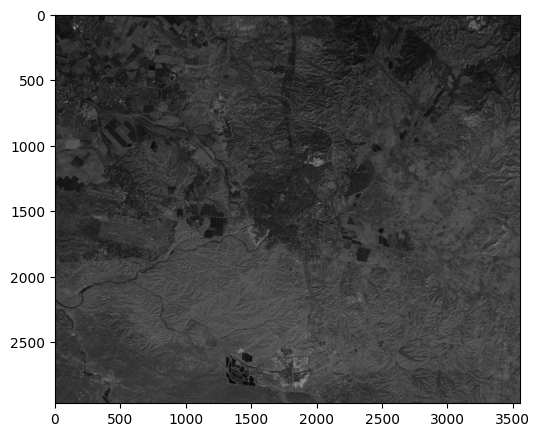
The resulting greyscale image can be displayed as follows:

rasterio.plot.show(greyscale, cmap='Greys_r');

Let’s move on to the second example, calculating an NDVI image. NDVI (Normalized Difference Vegetation Index) is a common remote sensing index, based on \(Red\) and Near-Infrared (\(NIR\)) reflectance, emphasizing green vegetation. The NDVI is defined as follows:

\[NDVI=\frac{NIR-Red} {NIR+Red}\]

Here is how we apply this formula to our Sentinel-2 image:

ndvi = (r[3] - r[2]) / (r[3] + r[2])
ndvi

array([[0.14      , 0.12658491, 0.14070147, ..., 0.29972248, 0.26146789,
        0.26984866],
       [0.15047085, 0.13375796, 0.13664341, ..., 0.38731061, 0.31643278,
        0.29107551],
       [0.14382877, 0.13605857, 0.14198535, ..., 0.5057818 , 0.40811003,
        0.32751092],
       ...,
       [0.09335508, 0.09921196, 0.09692956, ..., 0.05553949, 0.06145409,
        0.04998619],
       [0.0926337 , 0.09782162, 0.08964672, ..., 0.04974785, 0.05927031,
        0.04856187],
       [0.08914569, 0.09630249, 0.08908868, ..., 0.05008255, 0.05934991,
        0.04891524]])

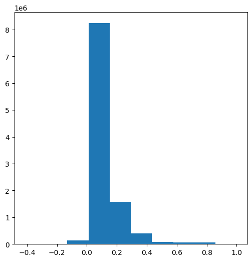
The possible range of NDVI values is between -1 and 1, however typical targes such as soil, built areas, and vegetation, produce positive NDVI values, between 0 and 1, whereas dense vegetation produces high NDVI values (up to ~0.8). Water bodies, clouds, and snow, produce zero or negative NDVI values. The distribution (see Histograms (numpy)) of NDVI values we got, where most values are between 0.05 and 0.30, is characteristic to dry areas with sparse vegetation cover:

plt.hist(ndvi.flatten());

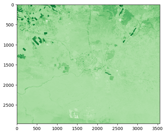
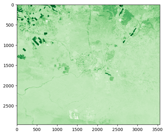
The following expression displays the NDVI image which we created, using the 'Greens' color palette. We can see that densely vegetated areas, such as agricultiral fields (top-left corner of the image), are emphasized due to their high NDVI values:

rasterio.plot.show(ndvi, cmap="Greens");

DEM calculations

Overview

There is a large number of specialized GIS functions and operators applicable to DEMs. These include, for example:

• Topographic indices, such as slope and aspect

• Flow accumulation, contributing area, and basin/channel delineation

• Visibility, line of sight, and visible area

This type of operations is beyond the scope of rasterio, but there are other, more spatialized third-party Python packages for DEM analysis. In this section, we are going to demonstrate calculation of topographic indices, namely topographic aspect, using the richdem package.

Note

Check out the documentation of richdem to get an idea of the other DEM-related operations available in this package: https://richdem.readthedocs.io/en/latest/intro.html.

richdem comes with its own functions to import and export data, named rd.LoadGDAL and rd.SaveGDAL, respectively. Accordingly, richdem defines its own class for storing rasters, called rdarray. We are not going to get into details about this data structure, because we already know how to the analogous operations (such as pre-processing, or examining the properties of rasters) using rasterio. Our strategy for working with richdem will be as follows:

• Import a DEM from a .tif file (which may have been prepared using rasterio) using rd.LoadGDAL

• Apply richdem functions as necessary

• Export the result using rd.SaveGDAL (perhaps for further processing with rasterio)

Topographic aspect

Our example to demontrate the workflow of richdem is calculating a topographic aspect raster. In the derived topographic aspect raster, the value of each pixel reflects the direction where the surface of that pixel (and its \(3\times3\) surrounding neighborhood) is facing, usually in decimal degrees (0-360). The ArcPro documentation has a good article named How Aspect works with more details about the topographic aspect calculation.

First, we load the 'carmel.tif' raster (see Writing single-band (int)) using function rd.LoadGDAL from the richdem package:

dem = rd.LoadGDAL('output/carmel.tif')

Here is what the resulting rdarray object looks like when printed. As you can see, it is very similar to a numpy array:

dem

rdarray([[-9999, -9999, -9999, ..., -9999, -9999, -9999],
         [-9999, -9999, -9999, ..., -9999, -9999, -9999],
         [-9999, -9999, -9999, ..., -9999, -9999, -9999],
         ...,
         [-9999, -9999, -9999, ..., -9999, -9999, -9999],
         [-9999, -9999, -9999, ..., -9999, -9999, -9999],
         [-9999, -9999, -9999, ..., -9999, -9999, -9999]], dtype=int16)

Importantly, the rdarray object keeps track of “No Data” value, which in our case is -9999:

dem.no_data

-9999.0

Now, we need to apply the richdem function for calculating topographic aspect given a DEM. This is done using rd.TerrainAttribute with the argument attrib='aspect':

aspect = rd.TerrainAttribute(dem, attrib='aspect')

Here is the result:

aspect

rdarray([[-9999., -9999., -9999., ..., -9999., -9999., -9999.],
         [-9999., -9999., -9999., ..., -9999., -9999., -9999.],
         [-9999., -9999., -9999., ..., -9999., -9999., -9999.],
         ...,
         [-9999., -9999., -9999., ..., -9999., -9999., -9999.],
         [-9999., -9999., -9999., ..., -9999., -9999., -9999.],
         [-9999., -9999., -9999., ..., -9999., -9999., -9999.]],
        dtype=float32)

For examining the output (or further processing it), we will use the more familiar rasterio methods. For that, we need to export the resulting aspect object, using rd.SaveGDAL:

rd.SaveGDAL('output/carmel_aspect.tif', aspect)

Then, we can “re-import” it with rasterio.open:

aspect = rasterio.open('output/carmel_aspect.tif')

We can now, for example, plot the aspect raster to see what it looks like:

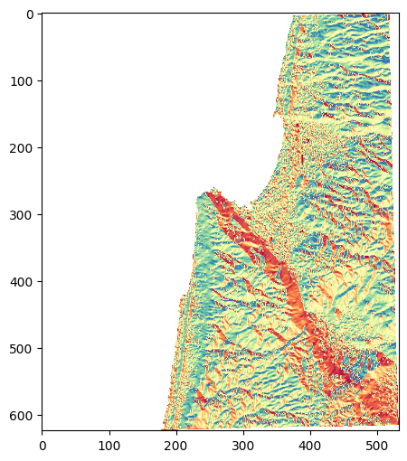
rasterio.plot.show(aspect, cmap='Spectral');

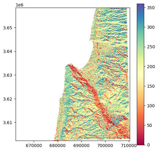
Here is another version of the plot, using a workaround to add a legend. That way, we can see that the aspect values are between \(0\) and \(360\) (degrees) as expected:

fig, ax = plt.subplots()
image_hidden = ax.imshow(aspect.read(1, masked=True), cmap='Spectral')
fig.colorbar(image_hidden, ax=ax)
rasterio.plot.show(aspect, ax=ax, cmap='Spectral');

Focal filtering

Our final example with rasters with rasters demonstrates a well-known third-party package called scipy. scipy is a broad-scope and established packages for scientific computing. One of the sub-domains which the package deals with is image processing. Typical image processing operations include filtering (which we demonstrate below), segmentation, and edge detection. Though image processing is not specific to spatial rasters, most operations are applicable and relevant when dealing with spatial data.

To work with scipy, as always, we first need to import it. The scipy is split to sub-packages addressing different domains. Each sub-module we want to work with needs to be imported separately, as if it is a standalone package. The scipy.ndimage sub-package (which we loaded earlier, see Loading raster packages), for example, includes the image processing-related functions, such as functions for different types of filters.

The most straightforward filtering function is ndimage.uniform_filter, where each pixel in the “filtered” image is the average of pixel values inside a moving window of a specified size. For example, window size of \(3\) implies that each pixel in the filtered image is the average of \(3\times3=9\) neighborhood centered on the “focal” pixel being calculated.

Here is how we can apply a uniform focal filter with a window size of 3 on the ndvi image we calculated earlier. Note that ndvi is the ndarray with the NDVI values:

ndvi3 = scipy.ndimage.uniform_filter(ndvi, 3)

The result ndvi3 is also an ndarray, of the same shape as ndvi. Only the values have changed. To understand how the calculation was carried out, we can compare the average of any particular \(3\times3\) neighborhood in the original raster:

ndvi[0:3, 0:3].mean()

0.13889236590152285

with the “focal” pixel value of that neighborhood in the filtered raster:

ndvi3[1, 1]

0.13889236590152285

The values are identical, as expected.

Displaying the filtered raster should appear more blurred than the original image. This is difficult to see in our last example, because the raster is relatively large and the focal window is relatively small:

rasterio.plot.show(ndvi3, cmap='Greens');

Exercise 10-f

• Try repeating the above with a larger filter size of 51 (instead of 3).

• Use rasterio.plot.show to see the result. The result should appear more blurred (Fig. 61).

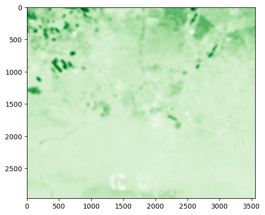
Fig. 61 Solution of exercise-10-f: Focal filter with window size of 51 applied on NDVI image

Note

There is a lot more to image processing using numpy and scipy than shown here. For example, check out the image processing tutorial. Also, check out the scikit-image package, which extends scipy.ndimage.

More exercises

Exercise 10-g

• Read the topographic aspect raster output/carmel_aspect.tif (see Topographic aspect).

• Replace “No Data” pixel values (-9999.) with np.nan.

• Reclassify (see Reclassifying) raster into four categories:

  • 0—North, \(aspect>315\) or \(aspect\leq45\)

  • 1—East, \(45<aspect\leq135\)

  • 2—South, \(135<aspect\leq225\)

  • 3—West, \(225<aspect\leq315\)

• Plot the reclassified image in the Jupyter Notebook (Fig. 62)

• Export the reclassified image to output/carmel_aspect_reclassified.tif and examine it in a GIS software (Fig. 63)

• Display the frequency (i.e., number of pixels) of each class in a barplot (Fig. 64). Use the .plot.bar method from pandas to draw the barplot.

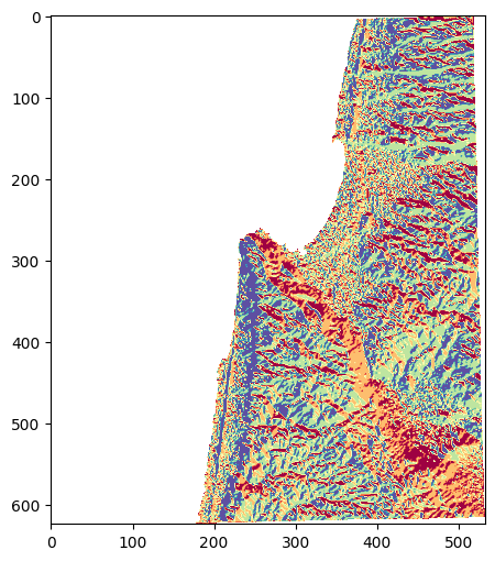
Fig. 62 Solution of exercise-10-g2: Reclassified aspect raster

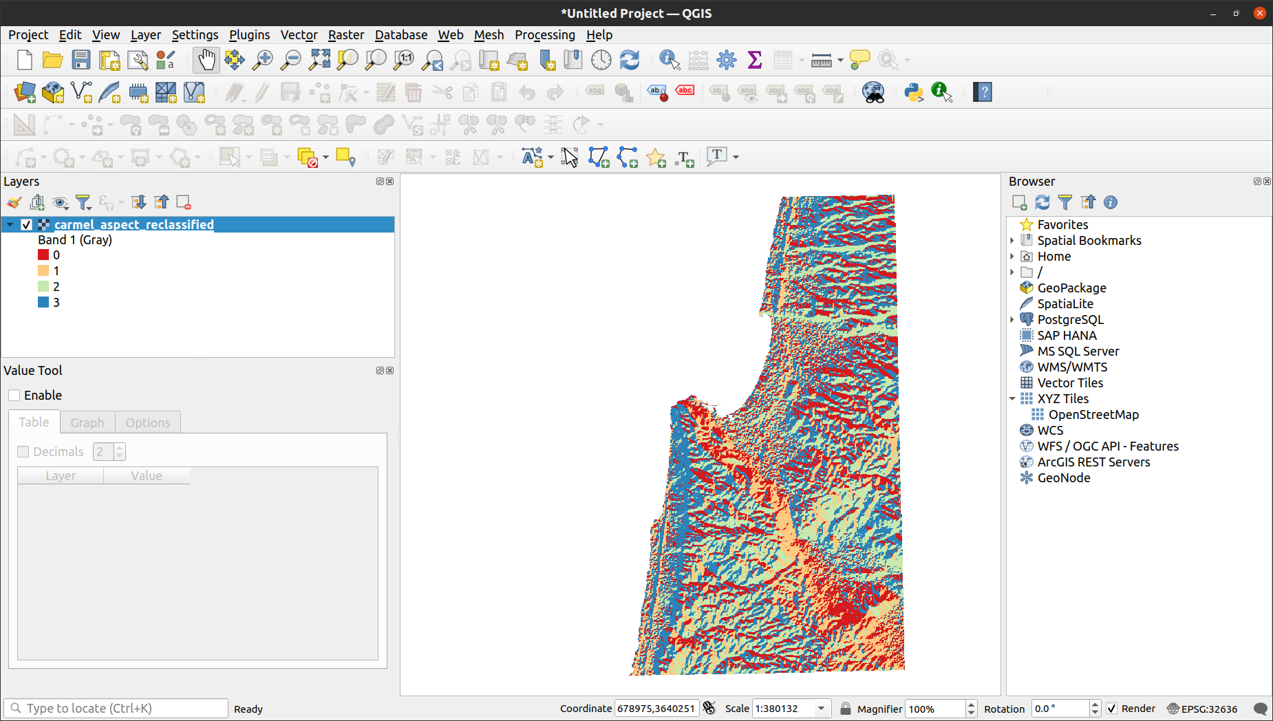
Fig. 63 Reclassified aspect image displayed in QGIS

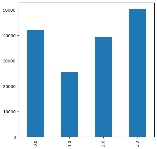
Fig. 64 Solution of exercise-10-g3: Frequency of topographic aspect classes

Exercise 10-e

• Read the Sentinel-2 multispectral image (output/sentinel2.tif) (see Stacking raster bands)

• Rescale the image values to the 0-1 range (see Rescaling)

• Calculate an Enhanced Vegetation Index 2 (EVI2) image, using the formula:

\[EVI2 = 2.5 * \frac{NIR - Red} {NIR + 2.4 * Red + 1}\]

• Plot the resulting image (Fig. 65)

• Draw a scatterplot of NDVI vs. EVI values (Fig. 66)

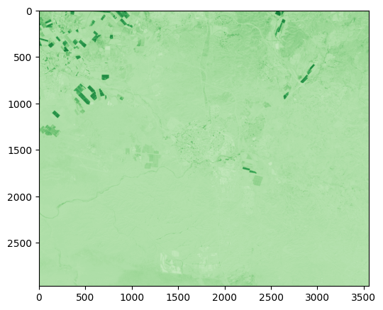
Fig. 65 Solution of exercise-10-h1: Enhanced Vegetation Index 2 image of the Beer-Sheva area

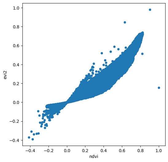
Fig. 66 Solution of exercise-10-h2: Association between NDVI and EVI2 indices

Exercise solutions

Solution 10-f

import rasterio
from rasterio.plot import show
import scipy.ndimage
src = rasterio.open("output/sentinel2.tif")
r = src.read()
r = r / 10000
r[r > 1] = 1
ndvi = (r[3]-r[2]) / (r[3] + r[2])
ndvi31 = scipy.ndimage.uniform_filter(ndvi, 51)
rasterio.plot.show(ndvi31, cmap="Greens");

Solution 10-g

import rasterio
import numpy as np
from rasterio.plot import show
# Read
src = rasterio.open('output/carmel_aspect.tif')
r = src.read(1)
# Set "No Data" to 'np.nan'
r[r == src.nodata] = np.nan
# Reclassify
s = r.copy()
s[(r > 315) | (r <= 45)] = 0
s[(r > 45) & (r <= 135)] = 1
s[(r > 135) & (r <= 225)] = 2
s[(r > 225) & (r <= 315)] = 3
# Write
dst = rasterio.open('output/carmel_aspect_reclassified.tif', 'w', **src.meta)
dst.write(s, 1)
dst.close()
# Plot
rasterio.plot.show(s, cmap='Spectral');

# Barplot
x = s.flatten()
x = pd.Series(x)
x = x.value_counts().sort_index()
x.plot.bar();

Solution 10-h

import rasterio
import pandas as pd
from rasterio.plot import show
# Read
src = rasterio.open('output/sentinel2.tif')
r = src.read()
# Rescale
r = r / 10000
# Calculate EVI2
L = 1
C1 = 6
C2 = 7.5
G = 2.5
blue = r[0, :, :]
red = r[2, :, :]
nir = r[3, :, :]
evi2 = 2.5 * (nir - red) / (nir + 2.4 * red + 1)
# Plot
rasterio.plot.show(evi2, cmap='Greens');

# Scatterplot of NDVI vs. EVI
ndvi = (r[3]-r[2]) / (r[3] + r[2])
dat = pd.DataFrame({
    'ndvi': ndvi.flatten(),
    'evi2': evi2.flatten(),
})
dat.plot.scatter(x='ndvi', y='evi2');