Chapter 12 Client-Side Geoprocessing
Last updated: 2018-11-11 20:44:59
12.1 Introduction
In Chapter 11, we used a spatial SQL query to load a subset of features from a PostGIS database on a web map. Specifically, we have performed a geoprocessing operation - finding the n-nearest points - using SQL. Notably, the operation was performed on the server (the CARTO database, in this case), and the result was returned to us via HTTP. Sometimes, it is more convenient to perform geoprocessing operations on the client, rather than on the server, for various reasons.
One reason to prefer client-side processing is that we may need the web page to be instantaneously responsive, as in a map with a layer which is continuously updated in response to user input (Figure 12.5). This is impossible to achieve this with a server: no matter how fast our internet connection is, there is usually going to be a noticeable lag due the time interval between sending the request and receiving the response. Another reason may be the relative simplicity and flexibility of using various algorithms and methods through JavaScript libraries, compared to the cost of setting up and managing a server with the same functionality.
The main disadvantage of client-side geoprocessing is that we are limited by the hardware constraints of the client. While the hardware of the server is (potentially) very powerful and in any case is under our control, the different clients who connect to our web page may have various hardware configurations. To make our website responsive, we should therefore limit client-side geoprocessing to relatively light-weight operations. Another constraint in client-side geoprocessing is that we are limited to JavaScript libraries and cannot rely on any other software or programming language (such as a PostGIS database).
In this Chapter we will see several examples of client-side geoprocessing operations, such as calculating Great Circle lines, point clustering and calculating heatmaps. All of these will be done in the browser, using JavaScript code, without requiring a dedicated server.
In the examples, we will use two different JavaScript libraries -
12.2 Geoprocessing with Turf.js
12.2.1 Overview
Turf.js is a JavaScript library for client-side geoprocessing. It includes a comprehensive set of functions, covering a wide range of geoprocessing tasks. The Turf.js library also has excellent documentation, including a small visual example for each of the functions.
As we will shortly see, the basic data type that Turf.js works with is GeoJSON. This is very convenient, because it means that any geoprocessing product can be immediately loaded on a Leaflet map with the L.geoJSON function, which we are well familiar with since Chapter 7. As for the other way around, we will also see that any existing Leaflet layer can be converted back to GeoJSON using the .toGeoJSON method, so that the resulting GeoJSON can then be passed to a Turf.js function for processing. As a result, we will sometimes have to go back and forth between Leaflet layer objects, which the Leaflet library understands, and GeoJSON objects, which the Turf.js library understands (Section 12.4.5).
In this Chapter, we will use seven different functions from the Turf library (Table 12.1). There are dozens of other functions which we will not use; you are invited to browse through the documentation to explore what kind of other tasks can be done with Turf.js.
| Function | Description |
|---|---|
turf.point |
Convert point coordinates to GeoJSON of type "Point" |
turf.greatCircle |
Calculate a Great Circle line |
turf.randomPoint |
Calculate random points |
turf.tin |
Calculate a Triangulated Irregular Network (TIN) |
turf.clusterEach |
Apply function on each subset of features |
turf.convex |
Calculate a Convex Hull polygon |
turf.clustersDbscan |
Perform DBSCAN clustering |
12.2.2 Including the Turf.js library
To use Turf.js on our web page we first need to include it using a <script> element. As always, the JavaScript file for this library can be included from a local copy, or from a CDN such as the following -
https://npmcdn.com/@turf/turf/turf.min.js
We will use a local copy stored in the js folder on our server, therefore adding the following <script> element inside the <head>. You can download the Turf.js file from above URL and place it in a local folder if you want to include a local copy in your web page.
<script src="js/turf.js"></script>12.3 Great Circle line
As a first experiment with Turf.js, we will use the library to calculate a Great Circle line, then display it on a Leaflet web map. A Great Circle line is the shortest path between two given points on the earth surface, taking the curvature of the earth into account (Figure 12.10). Through this example, we will demonstrate the way that Turf.js functions operate on GeoJSON objects.
All functions from the Turf.js package are loaded as methods of a global object named turf, thus sharing the turf. prefix. This is much like Leaflet functions start with L and jQuery functions start with $.
As an example, let’s open the documentation of the turf.greatCircle function. Here is a slightly modified code of the example given for the turf.greatCircle function in the documentation -
var start = turf.point([-122, 48]);
var end = turf.point([-77, 39]);
var greatCircle = turf.greatCircle(start, end);
- Open the basic map
example-06-02.htmlfrom Section 6.5.6- Add a
<script>element in the<head>for including the Turf.js library- Open the console and execute the above three expressions
What does this piece of code do? The first two expressions are using a convenience function named turf.point to convert pairs of coordinates into a GeoJSON object. The coordinates are assumed to be of the [lon, lat] form, same as in GeoJSON. Typing JSON.stringify(start) reveals the resulting GeoJSON for the first point -
{
  "type": "Feature",
  "properties": {},
  "geometry": {
    "type": "Point",
    "coordinates": [-122, 48]
  }
}
Note that the [-122, 48] coordinates passed to turf.point are now in the coordinates property of the GeoJSON. The output of typing JSON.stringify(end) would be identical, except for the coordinates which will be [-77, 39] instead of [-122, 48]. (Type JSON.stringify(end) in the console to see for yourself.)
The third expression uses the geoprocessing function turf.greatCircle to calculate the Great Circle line between the two points. The result is assigned to a variable named greatCircle. Here is the printout of JSON.stringify(greatCircle) -
{
  "type": "Feature",
  "properties": {},
  "geometry": {
    "type": "LineString",
    "coordinates": [
        [-122, 48],
        [-121.49670597260395, 48.006695584053034],
        [-120.9933027193627, 48.011192319649155],
        ...,
        [-77, 38.99999999999999]
    ]
  }
}
This is a "LineString" GeoJSON representing a Great Circle line. Most of the line coordinates array of the greatCircle object are omitted here, replaced with ... to save space.
- How many
[lon, lat]coordinate pairs is thegreatCircleline composed of?- Type the appropriate expression in the console to find out
When the above code section is executed in a web page with a Leaflet map object named map, the following expression can be used to draw the Great Circle line we just calculated on the map. We are using L.geoJSON to go from a GeoJSON object to a GeoJSON layer, then adding it on the map. Note that you need to zoom-in on the US to see the line, as it goes from Seattle to Washington, DC.
L.geoJSON(greatCircle).addTo(map);Similarly, we can draw markers at the start and end points as follows -
L.geoJSON(start).addTo(map);
L.geoJSON(end).addTo(map);
- Type these expressions in the console
- Make sure you see the Great Circle line and markers on the map
This is the general principle of working with most functions in Turf.js, in a nutshell: reshaping our data with Turf.js convenience functions, passing GeoJSON objects to Turf.js geoprocessing functions, and getting new GeoJSON objects in return.
We are now ready for two extended examples demonstrating the workflow of using Turf.js with Leaflet -
- In the first example, we will build a web map where a continuously updated TIN layer is generated while the user can drag any of the underlying points (Figure 12.5).
- In the second example, we will perform spatial clustering to detect and display distinct groups of rare species observations (Figure 12.8).
12.4 Continuously updated TIN
12.4.1 Overview
As our first extended use case of Turf.js, we are going to build a web map with a dynamic demonstration of TIN layers. The map will display a TIN layer generated from a set of randomly placed points. The user will be able to drag any of the points, observing how the TIN layer is being updated in real time (Figure 12.5).
We will go through several steps to accomplish this task -
- First, in
example-12-01.htmlwe are to going to generate random points and add them on a Leaflet map (Section 12.4.2) - Subsequently, in
example-12-02.htmlwe will generate a TIN layer on top of these points (Section 12.4.3) - Then, in
example-12-03.htmlwe will learn how to make a Leaflet marker draggable (Section 12.4.4) - Finally, in
example-12-04.htmlwe will make all of our random points draggable and binded to an event listener that updates the TIN layer in response to any of the points being dragged (Section 12.4.5).
12.4.2 Generating random points
The turf.randomPoint function from the Turf.js library can be used to generate GeoJSON with randomly placed points. When using the turf.randomPoint function, we need to specify -
- The number of points to generate
- A bounding box, defined using an array of the form
[lon0, lat0, lon1, lat1]
The turf.randomPoint function randomly places the specified number of points withing the given bounding box, and returns the resulting point layer as GeoJSON.
For example, in the following code section the first expression defines a bounding box coordinates array bounds, using the above four-element array structure that turf.randomPoint expects. In this case we are using the coordinates of the bounding box of Israel.
The second expression then generates 20 random points placed withing the bounding box. Note that the bounding box array needs to be passed as the bbox property inside the options parameters of turf.randomPoint. If we omit the options object, the random points will be generated in the default global extent, i.e. [-180, -90, 180, 90].
The third expression transforms the returned GeoJSON points to a Leaflet layer, then adds the layer on the map.
var bounds = [34.26801, 29.49708, 35.90094, 33.36403];
var points = turf.randomPoint(20, {bbox: bounds});
L.geoJSON(points).addTo(map);
To view the points, it is convenient to set the initial map extent to the same bounding box where the points were generated. In the following expression, we initialize the Leaflet map using a view-setting method called .fitBounds. The .fitBounds method automatically detects the appropriate map center and zoom level so that the given extent fits the map bounds. The .fitBounds method is sometimes more convenient than .setView, which was introduced in Section 7.4, where the extent is set based on map center and zoom level rather than a bounding box.
Confusingly, the .fitBounds Leaflet-map method and the turf.randomPoint function from Turf.js require different forms of bounding box specifications. Specifically, like all other Leaflet functions, .fitBounds uses the [lat, lon] ordering instead of [lon, lat]. Also, .fitBounds needs the two bounding box “corners” to be separated in two internal arrays. So -
- Leaflet needs a
[[lat0, lon0], [lat1, lon1]]bounding box - Turf.js needs a
[lon0, lat0, lon1, lat1]bounding box
This is the reason that the bounds array is “rearranged” in the following call to .fitBounds, when initializing our Leaflet map to the same extent where the random points are -
var map = L.map("map").fitBounds(
    [[bounds[1], bounds[0]], [bounds[3], bounds[2]]]
);
L.tileLayer(
    "http://{s}.tile.osm.org/{z}/{x}/{y}.png",
    {attribution: "© OpenStreetMap"}
).addTo(map);
Including the latter five expressions in a web page with a basic Leaflet map displays 20 randomly placed point markers (example-12-01.html), as shown on Figure 12.1.
FIGURE 12.1: example-12-01.html (Click to view this example on its own)
- Open
example-12-01.htmlin a new tab- Refresh the page several times - you should see the 20 points being randomly placed in different locations each time
12.4.3 Adding a TIN layer
A Triangulated Irregular Network (TIN) is a geometrical method of connecting a set of points in such a way that the entire surface is covered with triangles. TIN is frequently used in 3D modeling, as this method can be used to construct a continuous surface out of a set of 3D points. In Turf.js, the turf.tin function can be used to calculate a TIN layer given a set of points.
Like with the turf.greatCircle function shown above, both input and output of turf.tin are GeoJSON objects. In the case of turf.tin, the input should be a point layer, and the output is a polygonal layer with the resulting TIN.
To draw a TIN layer based on the random points points on our map, we can add the following expressions at the bottom of the <script> in example-12-01.html. You can also run the expressions in the console of example-12-01.html to see the TIN layer being added in “real-time” -
var tin = turf.tin(points);
L.geoJSON(tin).addTo(map);
As shown above, points is a GeoJSON object representing a set of 20 random points. The result of turf.tin(points) is the GeoJSON object with the calculated polygonal TIN layer, hereby assigned to a variable named tin. In the second expression, the TIN layer tin is added on the map exactly with L.geoJSON, the same way we added the points.
The resulting map, now with the calculated TIN (example-12-02.html), is shown on Figure 12.2.
FIGURE 12.2: example-12-02.html (Click to view this example on its own)
- Open
example-12-02.htmland refresh the page several times- You should see a different TIN layer each time, according to the random placement of the markers
12.4.4 Draggable circle markers
So far, in example-12-02.html (Figure 12.2), we created a web map with randomly generated points and their associated TIN layer. Refreshing the web page in this example gives a nice demonstration of the TIN algorithm - each time the page is refreshed the points are differently rearranged and the TIN layer is updated accordingly. An even nicer demonstration, though, would be if we could drag any of the points wherever we want, and watch the TIN layer being updated in real-time. Perhaps you are already familiar with this type of behavior from Google Maps, or other web applications for calculating map directions, where the user can drag the marker denoting an origin or a destination, and the calculated route is continuously updated in response (Figure 12.3).
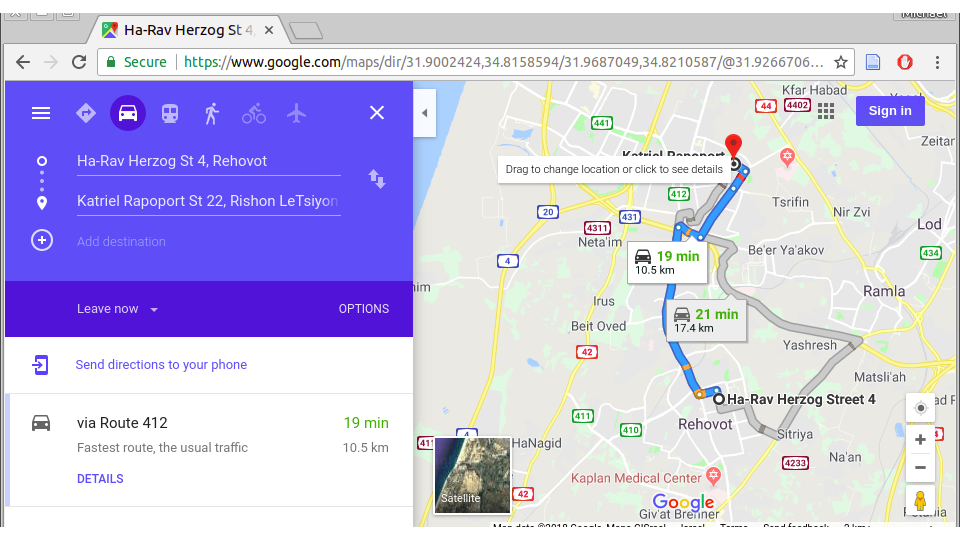
FIGURE 12.3: Draggable marker in the Google Maps Directions web application
The first thing missing to make our continuously-updated TIN is to make the 20 random markers actually draggable. This is exactly what we learn how to do in this section.
Going back to the basic map example from Section 6.5.6, adding the following code displays a draggable marker on the map. Note that the marker is placed in a manually defined location [32, 35] (of the form [lat, lon]), and has a popup message. Making the marker draggable requires setting its styling option draggable to true when creating it with L.marker.
var marker =
    L.marker([32, 35], {draggable: true})
    .bindPopup("This marker is draggable! Move it around...")
    .addTo(map)
    .openPopup();
On its own, the draggable marker is not very useful, because the TIN layer will not follow it once dragged. What we would like to do is make the TIN layer respond to every change in marker locations, by continuously updating itself.
To do that, we can add an event listener of type "drag" on each and every one of our 20 random markers. The function we define will be executed each time any of the markers is moved around. For now, we have just one draggable marker. To experiment with the "drag" event listener we can use a function that simply prints the current marker position, which can be accessed through a property named ._latlng that the marker has. The ._latlng property is an object with properties .lat and .lng, similarly to the .latlng event object property (Section 6.9).
marker.on("drag", function() {
     console.log(marker._latlng);
});
The result (example-12-03.html) is shown on Figure 12.4.
FIGURE 12.4: example-12-03.html (Click to view this example on its own)
- Open
example-12-03.htmland try dragging the marker around- Open the console to see the current location being printed each time the marker is being dragged
12.4.5 Continuous updating
Now, let’s combine the TIN example (Figure 12.2) with the draggable marker event listener example (Figure 12.4) to create a continuously-updated TIN. We are basically going to set {draggable: true} for all of the 20 randomly generated markers, then make the TIN layer update in response to any of those markers being dragged. The final result is shown on Figure 12.5.
To achieve this result, we will use a slightly modified approach for adding the points as well as the TIN layer. Instead of simply adding the points and the tin GeoJSON objects on the map right away, like we did in example-12-02.html -
var points = turf.randomPoint(20, {bbox: bounds});
var tin = turf.tin(points);
L.geoJSON(points).addTo(map);
L.geoJSON(tin).addTo(map);
We will set up two empty layers for the points and TIN, named pnt_layer and tin_layer, respectively. These layers will be referenced later on in the code. We are using L.layerGroup, which we learned about in Section 7.5.4, to create the empty layers.
var pnt_layer = L.layerGroup().addTo(map);
var tin_layer = L.layerGroup().addTo(map);
Next, we calculate the 20 random points -
var points = turf.randomPoint(20, {bbox: bounds});Remember that this time we don’t want to convert all points to a GeoJSON Leaflet layer with the default settings of L.geoJSON. Instead, we want to set the following -
- Make all of the markers draggable
- Add a
"drag"event listener to all markers, triggering the update of the TIN layer whenever any marker is dragged
This is why instead of using L.geoJSON with the default options, like we did in example-12-02.html -
L.geoJSON(points).addTo(map);We are now setting both the onEachFeature and pointToLayer options of L.geoJSON -
L.geoJSON(points, {
    onEachFeature: function(feature, layer) {
        layer.on("drag", drawTIN);
    },
    pointToLayer: function(geoJsonPoint, latlng) {
        return L.marker(latlng, {draggable: true});
    }
}).addTo(pnt_layer);
We are already familiar with using the onEachFeature option for adding event listeners to each GeoJSON feature. For example, in Chapter 8 we used this option to add "mouseover" and "mouseout" event listeners to highlight the towns polygons on mouse hover (Section 8.8.1). Here, we are adding a "drag" event listener. The function which will be executed on marker drag, named drawTIN, is yet to be defined (see below).
The other option pointToLayer is new, only briefly mentioned in the exercise for Chapter 8. This option is used to specify the way that GeoJSON points are to be translated to Leaflet layers, in case we want to override the default L.marker. In this case, we want to draw a marker with the {draggable: true} option, rather than the default marker.
Moving on, we now need to define the drawTIN function which is referenced inside the event listener. Each time a marker is dragged, the drawTIN function will be executed to calculate the new GeoJSON of the TIN layer, and replace the old TIN with the new one. Importantly, the new TIN layer is calculated based on the up-to-date pnt_layer to keep the points and the TIN in sync.
Here is the drawTIN function definition -
function drawTIN() {
    tin_layer.clearLayers();
    points = pnt_layer.toGeoJSON();
    tin = turf.tin(points);
    tin = L.geoJSON(tin);
    tin.addTo(tin_layer);
}
Essentially, each time a marker is dragged, the drawTIN function does the following things -
- Clears the
tin_layerlayer group, to remove the current TIN layer - Calculates the new TIN layer based on the current points in
pnt_layer - Adds the new TIN layer to the
tin_layerlayer group, thus drawing it on the map
These three things are accomplished through expressions 1, 3 and 5 in the drawTIN code body, respectively. What are expressions 2 and 4 for? They are necessary because of the above-mentioned fact that Turf.js functions only accept GeoJSON, and therefore cannot directly operate on Leaflet layers. Therefore we need to translate the Leaflet marker layer to GeoJSON in expression 2, then to translate the TIN GeoJSON back to a Leaflet layer in expression 4. The following code section repeats the internal code of drawTIN, this time with comments specifying the purpose of each expression -
tin_layer.clearLayers();         // Clear old TIN
points = pnt_layer.toGeoJSON();  // Layer -> GeoJSON
tin = turf.tin(points);          // Calculate new TIN
tin = L.geoJSON(tin);            // GeoJSON -> Layer
tin.addTo(tin_layer);            // Display new TIN
Finally, we need to execute the drawTIN function one time outside of the event listener. That way, the initial TIN layer will be displayed on page load, even if the user has not dragged any of the markers yet.
drawTIN();The resulting map (example-12-04.html) is shown on Figure 12.5. The screenshot shows how one of the points was dragged to the left, i.e. towards the west, and the TIN layer extended accordingly.
FIGURE 12.5: example-12-04.html (Click to view this example on its own)
12.5 Clustering
12.5.1 Overview
Clustering is the process of classifying a sample of observations into groups, so that objects in the same group (called a cluster) are more similar to each other than to those in other groups. With spatial clustering, similarity usually means geographical proximity, so that clustering aim is to group mutually proximate observations. In our second example with Turf.js, the final goal is to create a web map where clusters of nearby plant observations per species (i.e. populations), are detected using a clustering method called DBSCAN (see below) and displayed on a web map (Figure 12.8). We will approach this task in three steps -
- First, in
example-12-05.htmlwe will learn how to automatically apply the same script on subsets of GeoJSON features sharing the same value of a given property, such as observations of the same species (Section 12.5.2) - Second, in
example-12-06.htmlwe will learn to highlight the division of points into groups by drawing Convex Hull polygons around each group (Section 12.5.3) - Third, in
example-12-07.htmlwe will apply the DBSCAN clustering algorithm on the observation points per species to detect spatial clusters, and draw a Convex Hull polygon around each cluster (Section 12.5.4)
12.5.2 Processing sets of features
In the initial step of our clustering example, we are going to load observations of four Iris species from the plants table on CARTO, which we are familiar with from previous Chapters 9, 10 and 11. We are not doing any clustering just yet. The purpose of this example is to get familiar with the turf.clusterEach function. The turf.clusterEach function is used to apply a function on each group of GeoJSON features, whereas a group is defined through common values in one of the GeoJSON properties.
The script starts with constructing the URL for the SQL API and defining a styling function (getColor) for loading and setting the color of four Iris species observations.
// Set base URL
var url = "https://michaeldorman.carto.com/api/v2/sql?" +
    "format=GeoJSON&q=";

// Set SQL Query
var sqlQuery = "SELECT name_lat, the_geom " +
    "FROM plants WHERE " +
    "name_lat='Iris atrofusca' OR " +
    "name_lat='Iris atropurpurea' OR " +
    "name_lat='Iris mariae' OR " +
    "name_lat='Iris petrana'";


// Color function
function getColor(species) {
    if(species == "Iris mariae") return "yellow";
    if(species == "Iris petrana") return "brown";
    if(species == "Iris atrofusca") return "black";
    if(species == "Iris atropurpurea") return "orange";
}
The important part of the script, where our GeoJSON is loaded and added on the map, is shown below -
$.getJSON(url + sqlQuery, function(data) {
    turf.clusterEach(
        data,
        "name_lat",
        function (cluster, clusterValue, currentIndex) {
            L.geoJSON(cluster, {
                onEachFeature: function(feature, layer) {
                    layer.bindPopup(
                        "<i>" + clusterValue + "</i>"
                    );
                },
                pointToLayer: function(geoJsonPoint, latlng) {
                    return L.circleMarker(latlng);
                },
                style: function style(feature) {
                    return {
                        fillColor: getColor(clusterValue),
                        weight: 1,
                        opacity: 1,
                        color: "black",
                        fillOpacity: 0.5
                    };
                }
            }).addTo(map);
        }
    );
});
This is quite a long piece of code, which we will now explain in detail.
First, note that the function passed to $.geoJSON is not using L.geoJSON right away, like we did before. Instead, it contains an internal function call of the turf.clusterEach function, with the following form -
turf.clusterEach(
    data,
    "name_lat",
    function(cluster, clusterValue, currentIndex) {
        ...
    }
);
The turf.clusterEach function is another convenience function from Turf.js. It is used for iterating over groups of GeoJSON features sharing the same property values. The turf.clusterEach function accepts three arguments -
- The GeoJSON to iterate on, in our case it is the
dataobject received in$.getJSON, comprising GeoJSON with observations of four Iris species - The property name used for grouping, in our case it is
"name_lat", the Latin species name - A function to be applied on each set of features, with function parameters being the current set of features
cluster, the current property valueclusterValueand the current cluster indexcurrentIndex
In our case, the internal function passed to turf.clusterEach creates and draws a GeoJSON layer, using L.geoJSON. The function code uses the cluster and clusterValue parameters, which refer to the current set of GeoJSON features sharing the same value in the "name_lat" property, and the current value of the "name_lat" property, respectively.
$.getJSON(url + sqlQuery, function(data) {
    turf.clusterEach(
        data,
        "name_lat",
        function(cluster, clusterValue, currentIndex) {
            L.geoJSON(cluster, {
                ... // What to do with each set of features
            }).addTo(map);
        }
    );
});
Eventually, the code loads all observations of four Iris species (see SQL query above), then iterates over the four groups sharing the same species name. The iteration sequentially adds the observations of each species on the map.
For example, note that when adding circle marker popups we are using the following expression which refers to the current "name_lat" property -
layer.bindPopup("<i>" + clusterValue + "</i>");You may wonder why do we need to split the GeoJSON with turf.clusterEach, in the first place, rather than just add it at once to the map, like we used to do in previous Chapters -
$.getJSON(url + sqlQuery, function(data) {
    L.geoJSON(data, {
        ... // What to do with the entire GeoJSON
    }).addTo(map);
});
In this example, the the latter approach is indeed preferable since it is shorter and more simple. For the styling function which sets the marker color, it does not matter whether the GeoJSON is split to groups or loaded at once: the styling and popup content of a given species observation can be made specific on its name_lat value either way (see Chapter 8). However, this is just a preparation for what we do in the next two sections, where it is indeed required to treat each species separately, as we will be drawing a Convex Hull polygon around each species (Figure 12.7) or detection sub-populations using the DBSCAN clustering algorithm (Figure 12.8).
Additionally, note that when loading the GeoJSON we are using the pointToLayer option. As shown in Section 12.4.5 above, the pointToLayer option controls the way that GeoJSON points are translated to Leaflet shapes. Recall that in the previous example (example-12-04.html) we used pointToLayer to make our markers draggable (Figure 12.5). In the present example, the purpose of using pointToLayer is to override the default marker display, using circle markers instead of ordinary ones. The advantage of circle markers is that they can then be colored according the clusterValue, which refers to the name_lat property of the current group, so that observations of the different species are distinguished by their color.
...
pointToLayer: function(geoJsonPoint, latlng) {
    return L.circleMarker(latlng);
},
...
The resulting map (example-12-05.html) shows the observations of four Iris species. Each species is displayed with differently colored circle markers (Figure 12.6).
FIGURE 12.6: example-12-05.html (Click to view this example on its own)
12.5.3 Adding a Convex Hull
A Convex Hull is the smallest convex geometrical shape, typically a polygon, enclosing a given set of points. One of the uses of a Convex Hull in data visualization, in general, and in geographical mapping, in particular, is to highlight the geographical extent that a group of observations occupies, possibly to distinguish between extents occupied by other groups. In other words, Convex Hull polygons are a useful and convenient way of highlighting the division of individual observations into groups.
In our second step of the clustering example (this Section), we will experiment with drawing Convex Hull polygons to highlight the extent that each Iris species occupies in space overall (Figure 12.7). In the third and final step (next Section 12.5.4), we will determine internal observation clusters within each species, and draw Convex Hull polygons around each cluster within each species (Figure 12.8).
To draw a Convex Hull polygon around all observations of each species, all we need to do is add the following code within the turf.clusterEach iteration from example-12-05.html -
var ch = turf.convex(cluster);
L.geoJSON(ch, {
    style: function style(feature) {
        return {
            fillColor: getColor(clusterValue),
            weight: 1,
            opacity: 1,
            color: "black",
            fillOpacity: 0.5
        };
    }
}).addTo(map);
The code takes the current set of points cluster, calculates their Convex Hull polygon with turf.convex, then adds that polygon on the map with L.geoJSON. Remember that cluster is consecutively assigned with a different set of features for each species as part of the turf.clusterEach iteration. Since the code for calculating the Convex Hull and drawing it on the map is placed inside the iteration, a separate Convex Hull polygon is calculated per species, thus highlighting the species distribution ranges (Figure 12.7). Conveniently, we are using the same styling function getColor for both circle markers and Convex Hull polygons, so that their fill colors are the same.
FIGURE 12.7: example-12-06.html (Click to view this example on its own)
12.5.4 DBSCAN clustering
In spatial clustering, we aim at detecting groups of nearby observations which are close to each other, but further away from other observations. In the Iris example above, we may wish to detect spatial clusters, representing separate populations, within each of the species. To do that, we will experiment with a clustering technique called Density-Based Spatial Clustering of Applications with Noise or DBSCAN.
DBSCAN is a density-based clustering method, which means that points that are closely packed together are assigned into the same cluster and given the same ID. The DBSCAN algorithm has two parameters which the user needs to specify -
- \(\varepsilon\) - the maximum distance between points to be considered within the same cluster
- \(minPts\) - the minimal number of points required to form a cluster
In short, all groups of at least \(minPts\) points, where each point is within \(\varepsilon\) or less from at least one other point in the group, are considered to be a separate cluster and assigned with a unique ID. All other points are considered “noise”, and are not assigned with an ID.
The turf.clustersDbscan function is an implementation of the DBSCAN algorithm in Turf.js. The function accepts an input point layer and returns the same layer with a new property named "cluster". The "cluster" property contains the cluster ID assigned using DBSCAN. Noise points are not assigned with an ID and thus are not given a "cluster" property.
The first parameter of the turf.clustersDbscan function is maxDistance (\(\varepsilon\)), which determines what is the maximal distance between two points to be considered within the same cluster, in Kilometers. In our example (see below) we will use a maximal distance 10 Kilometers. The minPoints (\(minPts\)) parameter has a default value of 3, which we will not override.
To experiment with turf.clustersDbscan, you can execute the following expression in the console of example-12-01.html. This will apply DBSCAN with a maxDistance value of 10 Kilometers on the 20 randomly generated points.
turf.clustersDbscan(points, 50);
- Examine the result of the above expression to see which of the 20 random points were assigned to a cluster and given a
clusterproperty with a numeric value (i.e. the ID)- Try increasing and decreasing the
maxDistancevalue 0f50and executing the expression again- As
maxDistancegets larger, all points will tend to aggregate into the same single cluster. Conversely, asmaxDistancegets smaller, it will be more “difficult” for clusters to created, which means that more and more points will be classified as noise
Back to our Iris species example. When applying the DBSCAN algorithm on the observations of a given species, those observations which are not considered as noise are going to be associated with a "cluster" property. We can then iterate over the clusters to add a Convex Hull around each population. Practically, this can be accomplished by adding another, internal, turf.clusterEach iteration through all of the features sharing the same "cluster" attribute value within a given species.
To achieve the latter, we replace the code section shown above for adding Convex Hull polygons based on species identity, with the following code section for adding Convex Hull polygons based on DBSCAN clustering -
clustered = turf.clustersDbscan(cluster, 10);
turf.clusterEach(
    clustered,
    "cluster",
    function(cluster2, clusterValue2, currentIndex2) {
        var ch = turf.convex(cluster2);
        L.geoJSON(ch, {
            style: function style(feature) {
                return {
                    fillColor: getColor(clusterValue),
                    weight: 1,
                    opacity: 1,
                    color: "black",
                    fillOpacity: 0.5
                };
            }
        }).addTo(map);
    }
);
We leave it as an exercise for the reader to go over the code, as we are essentially combining the methods already covered in the previous two examples.
The final result (example-12-07.html) is shown on Figure 12.8. It is now evident, for instance, how Iris petrana (the south-eastern species shown in brown) observations are clustered in one place, while the distribution range of the other three species are divided into two or three distinct populations separated by at least 10 Kilometers (Figure 12.8).
FIGURE 12.8: example-12-07.html (Click to view this example on its own)
- Add popups for the Convex Hull polygons to display the species name and the cluster ID when clicked
- Modify the maximal distance and check how the division into populations changes
12.6 Heatmaps with Leaflet.heat
Turf.js is one of the most comprehensive client-side geoprocessing JavaScript libraries, but it is not the only one. The Leaflet.heat library, for example, is a geoprocessing plugin for the Leaflet library. The term “plugin”, in this context, means that Leaflet.heat is an extension of the Leaflet library and thus cannot be used without Leaflet, unlike Turf.js which is an independent library that can be used with Leaflet or with any other library, or even on its own. Also unlike Turf.js, which is a general-purpose geoprocessing library, Leaflet.heat does just one thing - drawing a heatmap to display the density of point data. The Leaflet.heat plugin is one of many plugins created to extend the core functionality of Leaflet. In Chapter 13 we will work with another Leaflet plugin called Leaflet.draw.
Drawing individual points can be visually overwhelming, slow, and hard to comprehend when there are too many points. Heatmaps are a convenient way of conveying the distribution of large amounts of point data. A heatmap is basically a way to summarize and display point density, instead of showing each and every each individual point. Technically speaking, a heatmap uses two-dimensional Kernel Density Estimation (KDE) to calculate a smooth surface representing point density.
The following example (example-12-08.html) draws a heatmap of all rare plant observations from the plants table on CARTO. Overall, there are 23,827 points in the plants table; drawing markers, or even the simpler circle markers, for such a large amount of points is usually not a good idea. First, it may cause the browser to become unresponsive due to computational intensity. Second, it is usually difficult to pick the right styling (size, opacity, etc.) for each point so that dense locations are clearly distinguished on the various map zoom levels the user may choose. This is where the density-based heatmaps become very useful. Particularly, the Leaflet.heat library automatically re-calculates the heatmap for each zoom level, allowing the user to conveniently explore point density on both large and small scales.
To use the Leaflet.heat library we first need to load it. Again, we will use a local copy -
<script src="js/leaflet.heat.js"></script>Which can be downloaded, or directly referenced, using the following URL -
https://leaflet.github.io/Leaflet.heat/dist/leaflet-heat.jsNext, when loading the plant observations GeoJSON we need to convert it to an array of [lat, lon, intensity] arrays, since this is the data structure the Leaflet.heat library expects. The intensity value can be used to give different weights to each point.
[
    [lat, lon, intensity],
    [lat, lon, intensity],
    [lat, lon, intensity],
    ...
]
There are many ways to go from a point layer GeoJSON to the above array structure. The code section below shows one way to do it, using the $.each iteration method of jQuery (Section 4.11). The $.each iteration goes over the features of a GeoJSON object named data, such as the result of a CARTO SQL API request obtained with $.getJSON. For each of the features, the latitude and longitude are extracted into an array of the form [lat, lon], along with the constant intensity value of 0.5 which gives all points equal weights when calculating density. When the iteration ends, we have an array named locations, containing 23,827 triplets of the form [lat, lon, intensity].
var locations = [];
$.each(data.features, function(index, value) {
    var coords = value.geometry.coordinates;
    var location = [coords[1], coords[0], 0.5];
    locations.push(location);
});
Once the locations array is ready, we can run the L.heatLayer function on the array to create the heatmap layer, then add it on our map. The additional parameters define the radius of each point on the map (i.e. the smoothing kernel width) and the minimal heatmap opacity.
L.heatLayer(locations, {radius: 20, minOpacity: 0.5}).addTo(map); The result (example-12-08.html) is shown on Figure 12.9.
FIGURE 12.9: example-12-08.html (Click to view this example on its own)
12.7 Exercise
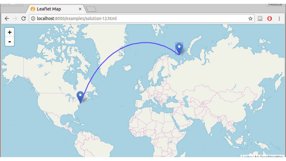
FIGURE 12.10: solution-12.html