Chapter 9 Databases
Last updated: 2018-11-11 20:44:59
9.1 Introduction
In Chapters 7 and 8, the data we used in web maps were stored in GeoJSON files on the server. This is a viable approach when our data are relatively small and not constantly updated. When this is not the case, however, using only GeoJSON can become limiting.
For example, loading large datasets from GeoJSON becomes prohibitive, because the entire file needs to be transferred through the network, even if we want display just some of the content, for example by subsetting the layer in the JavaScript code after it has been received. It is obviously unreasonable to have the user wait until tens or hundreds of Megabytes are being received, in the meanwhile seeing an empty map. Processing very large amounts of data will probably also make the browser unresponsive. A natural solution is to use a database. Unlike a file, a database can be queried to request just the required portion of information each time, thus transferring and processing manageable amounts of data.
Another limitation of using GeoJSON files becomes relevant when the data are constantly updated, and used for other purposes rather than just being displayed on our particular web map. For example, we may wish to build a web map displaying real-time municipal events, but have the data constantly updated or edited (e.g., by the municipality staff) and/or used in various contexts (e.g. viewed in GIS software by other professionals). Again, a natural solution is to use a database, shared between numerous concurrent connections for viewing and editing the data, through many types of different interfaces. Our web map, making use of one such concurrent connection, will therefore be synchronized with the database contents so that the displayed information is always up-to-date.
The next three Chapters (Chapter 9, 10 and 11) introduce the idea of loading data from a spatial database to display them on an interactive map, while dynamically filtering the data to transfer just the portion that we need. That way, we are freed from the limitation regarding the amount of data “behind” the web map. In other words, the database that stands behind our web map can be very large in size, yet the web map will stay responsive, thanks to the fact that we load subsets of the data each time, based on what the user chooses to see. In this Chapter (Chapter 9) we introduce the concepts and technologies that enable a Leaflet map to load data from a spatial database. In the next two Chapters, we go through examples of using non-spatial (Chapter 10) and spatial (Chapter 11) database queries for loading subsets of data from a database.
It should be mentioned that Web Map Services (WMS) comprise an alternative solution for displaying large, up-to-date, amounts of data on a web map, however this solution is beyond the scope of this book. In short, with a WMS we are using a GIS database to build on-demand raster tiles. The server generates custom tiles based on the parameters it is given, so that the user has control on displayed content, such as choosing which layers to display. This is unlike pre-compiled tile datasets such as those introduced in Section 6.5.5, and used as base layers in the last two Chapters, since the latter are fixed and cannot be dynamically generated based on user input.
There are valid use cases for both the database and WMS approaches. Basically, the database approach works better when working with vector layer that the user interacts with, which is made possible by the fact that the server can send raw data (such as GeoJSON) and we can control the way that data are displayed on the client using JavaScript code. The WMS approach works better when our data are very complex and have elaborate symbology. In such case it makes sense to have a dedicated map server with specialized software to build raster images with the displayed content, and send them to the client to be displayed as-is. There is an official tutorial on using WMS with Leaflet, where you can see a concrete example.
9.2 What is CARTO?
9.2.1 The CARTO platform
A problem that immediately arises regarding retrieval of spatial data from a database onto a web map, is that client-side scripts cannot directly connect to a database. A dynamic server, which we mentioned in Section 5.4.3, is the solution. On the dynamic server, server-side scripts, which indeed can connect to the database, are used to query the database and send the data back to the client. In fact, the need to send information from a database to the browser is one of the main motives for setting up a dynamic server.
In this book we focus on client-side solutions, so we will not be dealing with setting up our own dynamic server coupled with a database. Instead, we will use a cloud-based service by a company called CARTO.
![]()
The CARTO platform provides several cloud computing GIS and Web mapping services. The most notable service, and the one we are going to use in this book, is the SQL API (Section 9.7). CARTO allows you to upload your own data into a managed spatial database, while CARTO’s SQL API allows you to interact with that database. In other words, CARTO takes care of setting up and maintaining a spatial database, as well as server-side components to make that database reachable through HTTP requests.
In this Chapter we will introduce the CARTO platform, and the technologies it is based on: spatial databases (Section 9.4), SQL (Section 9.6) and the SQL API (Section 9.7). Towards the end of the Chapter, we will see how CARTO can be used for querying and displaying data from a database on a Leaflet map (Section 9.8). In the next two Chapters we will dig a little deeper into different types of queries and their utilization in web mapping. In Chapter 10 we will see an example of non-spatial, attribute-based filtering of data based on user input from a dropdown menu. In Chapter 11 we will see an example of using spatial queries to retrieve data based on proximity to a clicked location.
9.2.2 Alternatives to CARTO
CARTO is a commercial service that comes at a price, though at the time of writing there is an option called Student Developer Pack which includes a 2-year free CARTO account.
It is worth mentioning that the CARTO platform is open-source. In principle, it can be installed on any computer to replicate almost the entire functionality of CARTO for free. The installation and maintenance is quite complicated though. A minimal configuration, with a simple dynamic server, a database, and an SQL API can be set up (relatively) more easily. The online version of the book includes an additional supplement with instructions for one way to do that, using Node.js and PostgreSQL/PostGIS. This will not be covered in the book, but it is important to be aware that no matter how convenient CARTO is, if some day we need to cut costs and manage our own server for the tasks covered in the next few Chapters - it can be done. All examples where a CARTO database is used are also given in an alternative version, using the custom setup instead of CARTO. The latter are marked with -s, as in example-09-01.html and example-09-01-s.html (Appendix B).
9.3 Databases
Before we begin using the CARTO platform, we need to introduce several concepts and technologies it involves -
- Databases
- Spatial databases
- PostGIS
- SQL
- API
The term database describes an organized collection of data. A database stores data, but also facilitates indexing, searching, and querying the data, as well as modifying and adding data. The most established and commonly used databases follow the relational model, where the records are organized in tables, and the tables are usually associated with one another via common columns or keys (Figure 9.1).
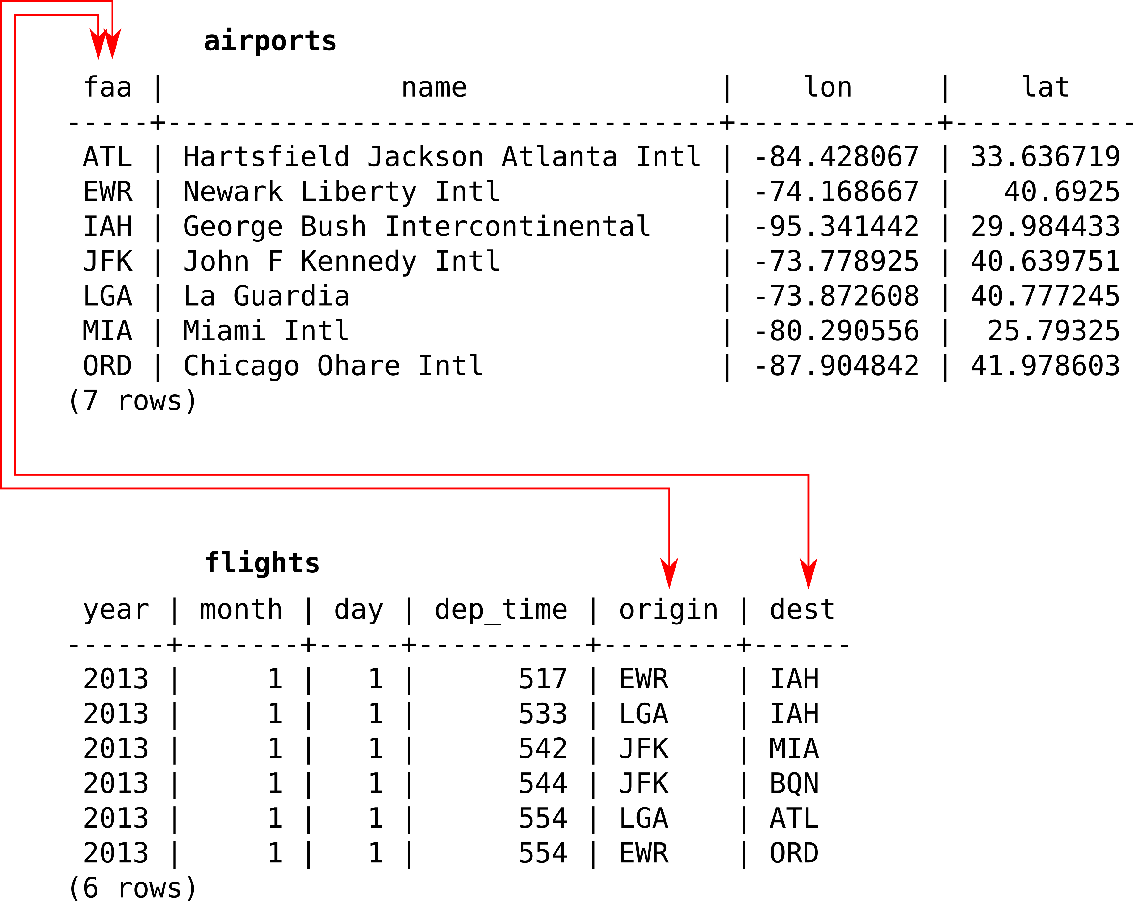
FIGURE 9.1: An example of a relational database with two tables
Database queries, including both ordinary and spatial ones, are expressed in a language called SQL (Section 9.6).
9.4 Spatial databases
A spatial database is a database that is optimized to store and query data that represents objects defined in a geometric space.
Regarding the storage part, plainly speaking, the tables in a spatial database have a special type of geometry column, which holds the geometric component of that specific record, i.e. the geometry type and the coordinates. This may sound familiar - recall the geometry GeoJSON types (Section 7.2.2), which represent just the geometric part of a feature. The similarity between the geometry column and the GeoJSON geometry types in not incidental, but due to the fact that both are based on the Simple Features standard which we mentioned in Section 7.2.1. The difference is that in a spatial database, the geometries are usually encoded in a format called Well-Known Binary (WKB), a binary version of the Well-Known Text (WKT) format (also mentioned in Section 7.2.1), rather than in the GeoJSON format.
In addition to geometry storage, spatial databases define special functions that allow for queries based on geometry. This means we can use the database to make spatial numeric calculations (e.g. geographical distance), retrieve data based on location (e.g. K-nearest neighbors), or create new geometries (e.g. the centroid of a geometry). These are called spatial queries, since they involve the spatial component of the database, i.e. the geometry column of at least one table. The concept is very similar to spatial operators and functions used in GIS software, such as the Select by Location tool in ArcGIS.
Some common open-source spatial databases include -
- PostgreSQL/PostGIS (used by CARTO)
- SQLite/SpatiaLite
- MySQL
There are also a large number of proprietary databases that support spatial data, such as -
- Oracle Spatial
- ESRI ArcSDE
- ESRI Geodatabase
These are just some of the most popular spatial databases, though there are many more.
9.5 What is PostGIS?
PostGIS is a popular extension for the PostgreSQL database, making the PostgreSQL/PostGIS combination a spatial database (Obe and Hsu 2015). In other words, a PostgreSQL database having the PostGIS extension enabled allows for storage of spatial data and execution of spatial SQL queries (Section 9.6.4 below) to be performed. At the moment, the PostgreSQL/PostGIS combination makes the most powerful open-source spatial database available. PostgreSQL with the PostGIS extension will be referred to as PostGIS from now on, for simplicity.
As both programs are free and open-source, you can install PostGIS on your computer and set up your own database. However, running a database requires some advanced setup and maintenance, which is outside the scope of this book. As mentioned above, the CARTO platform provides a cloud-based PostGIS database as a service, which we are going to use in this book.
9.6 What is SQL?
9.6.1 Overview
SQL is a language for writing statements to query or to modify tables stored in a relational database, whether spatial or non-spatial. Using SQL you can perform many types of tasks: selection, joins, insertions, updates, etc. SQL statements can be executed in many types of database interfaces, from command lines, through database administrative consoles in GIS software, and to APIs that connect to the database through HTTP such (such as CARTO). You may already be familiar with SQL syntax from GIS software, such as ArcGIS and QGIS, where SQL can be used to select features from a layer.
Using CARTO, we will experiment with writing SQL queries to extract data from a cloud-based database, and displaying these data on Leaflet map. That way we will become familiar with the whole idea of querying spatial databases from the web mapping perspective. Hopefully, this introduction will be of use if, later on, you decide to go deeper into the subject and set up your own spatial database server.
SQL, as you can imagine, is a very large topic. The syntax of SQL is not the focus of this book, so we will not go deeply into details nor will we cover the whole range of query types that can be used for various tasks. During the following Chapters, we will only meet about ~5-6 relatively simple types of SQL queries, most of which are briefly introduced below. This will be enough for our purposes, and you will be able to modify these statements to apply the same type of queries to different data, even if you have never used SQL before.
In the examples that follow, we will demonstrate a few types of SQL queries on a database that contains just one table named plants. The plants table contains rare plant observations in Israel. The data source of this table is the Endangered Plants of Israel website by the Israel Nature and Parks Authority. These examples are just for illustration and are not meant to be replicated in a console or command line, since we are not setting up our own database. However, shortly you will be able to apply them through the CARTO platform (Section 9.7 below).
Each row in the plants table represents an individual observation of a rare plant species. The table has different columns describing each observation, such as -
id- Observation IDname_lat- Latin species nameobsr_date- Observation dategeometry- The location (i.e. the geometry column)
9.6.2 Non-spatial queries
The most basic SQL statement is a SELECT statement. A SELECT statement requests data from a database, possibly filtered on various criteria, supplemented with new columns resulting from table joins or transformations, and so on. For example, we can use the following SELECT query to get a subset of the plants table, with just three of the above columns: id, name_lat and obsr_date, where the Latin species name is equal to the specific value 'Anticharis glandulosa'.
SELECT id, name_lat, obsr_date
  FROM plants
  WHERE name_lat = 'Anticharis glandulosa';
By convention, SQL keywords are written in uppercase, while specific values such as column names are written in lowercase. This is not strictly required, as SQL is not case-sensitive, unlike JavaScript which is case-sensitive. Spaces and line breaks are ignored in SQL, like in JavaScript. The query ends with the ; symbol.
Note that the queried column names are listed after the SELECT keyword, the table name is specified after FROM and the condition for filtering returned records is constructed after the WHERE keyword. In this case name_lat = 'Anticharis glandulosa' means “return all records where the value of name_lat is 'Anticharis glandulosa'”.
If we had access to a PostGIS database with the plants table and would type the above SQL query through its command line interface (called psql), the following textual printout of a small table would appear inside the command line. Note that the last line is not part of the result but only specifies the number of rows returned by the database.
   id   |       name_lat        | obsr_date
--------+-----------------------+------------
 339632 | Anticharis glandulosa | 1988-03-18
 359135 | Anticharis glandulosa | 2012-12-15
 367327 | Anticharis glandulosa | 2012-12-15
(3 rows)
According to this result we can tell that there are only three observations of 'Anticharis glandulosa' in the plants table.
9.6.3 The geometry column
As mentioned earlier, the distinctive feature of a spatial database is that its tables may contain a geometry column, describing the spatial location of each respective database record (i.e. table row). The geometry column usually contains binary code which is an encoded version of the Well-Known Text (WKT) format, known as Well-Known Binary (WKB). The binary compression is conventionally used to reduce the required storage space for the database.
For example, the geometry column in our particular plants table is named geometry. The following query returns the contents of three columns from the plants table, the “ordinary” id and name_lat columns, as well as the geometry column named geometry. The query is also limited to the first five records with the LIMIT 5 part -
SELECT id, name_lat, geometry
  FROM plants
  LIMIT 5;
Here is the printout we would see on the command line in this case -
   id   |    name_lat    |                  geometry
--------+----------------+--------------------------------------------
 321432 | Iris haynei    | 0101000000520C906802D741400249D8B793624040
 321433 | Iris haynei    | 0101000000D235936FB6D34140C6151747E55E4040
 321456 | Iris atrofusca | 01010000001590F63FC0984140EDB60BCD75723F40
 321457 | Iris atrofusca | 0101000000672618CE35984140357C0BEBC6833F40
 321459 | Iris vartanii  | 0101000000E6B0FB8EE19141405D6E30D461793F40
(5 rows)
It is evident the WKB strings make no sense to the human eye. However, WKB can always be converted to its textual counterpart WKT, using the ST_AsText operator, as demonstrated in the next slightly modified version of the above SQL query.
SELECT id, name_lat, ST_AsText(geometry) AS geom
  FROM plants
  LIMIT 5;
The only change is that we replaced the geometry part with ST_AsText(geometry), thus transforming the column from WKB to WKT. The AS geom part is used to rename the new column to geom (otherwise it would get a default name such as st_astext).
Here is the resulting table, with the geometry column transformed to its WKT representation and renamed to geom -
   id   |    name_lat    |            geom
--------+----------------+----------------------------
 321432 | Iris haynei    | POINT(35.679761 32.770133)
 321433 | Iris haynei    | POINT(35.654005 32.741372)
 321456 | Iris atrofusca | POINT(35.193367 31.44711)
 321457 | Iris atrofusca | POINT(35.189142 31.514754)
 321459 | Iris vartanii  | POINT(35.139696 31.474149)
(5 rows)
Similarly, we can convert the WKB geometry column to GeoJSON, which we are familiar with from Chapter 7. To do that, we simply use the ST_AsGeoJSON operator instead of the ST_AsText operator, as shown below.
SELECT id, name_lat, ST_AsGeoJSON(geometry) AS geom
  FROM plants
  LIMIT 5;
Here is the result, with the geometry column now given in the GeoJSON format -
   id   |    name_lat    |                         geom
--------+----------------+------------------------------------------------------
 321432 | Iris haynei    | {"type":"Point","coordinates":[35.679761,32.770133]}
 321433 | Iris haynei    | {"type":"Point","coordinates":[35.654005,32.741372]}
 321456 | Iris atrofusca | {"type":"Point","coordinates":[35.193367,31.44711]}
 321457 | Iris atrofusca | {"type":"Point","coordinates":[35.189142,31.514754]}
 321459 | Iris vartanii  | {"type":"Point","coordinates":[35.139696,31.474149]}
(5 rows)
The last two outputs tell us that the the plants table, or at least its first five records, contains geometries of type Point (Table 7.1).
9.6.4 Spatial queries
The geometry column can be used to apply spatial operators on our table, just like in GIS software. Much like general SQL (shown above), the syntax of spatial SQL queries is a very large subject, and mostly beyond the scope of this book. Nevertheless, in Chapter 11 we will experiment with the following specific type of a spatial query, which returns the nearest records from a given point.
The following example returns the nearest five observations from the plants table based on distance to the specific point [34.810696, 31.895923] (as in the [lon, lat]). Basically, the plants table is ordered according to the proximity of its geometries to (34.810696, 31.895923), then the top five records are returned.
SELECT id, name_lat, ST_AsText(geometry) AS geom
  FROM plants
  ORDER BY
    geometry::geography <->
    ST_SetSRID(
      ST_MakePoint(34.810696, 31.895923), 4326
    )::geography
  LIMIT 5;
The selection of top five records is done using the LIMIT 5 part. What’s new here is the part after the ORDER BY keyword, where we calculate all distances from plants points to a specific point [34.810696, 31.895923], and use these distances to order the table. We will elaborate on this part in Chapter 11.
Here is the result, with the five nearest observations to [34.810696, 31.895923] -
   id   |       name_lat       |            geom
--------+----------------------+----------------------------
 341210 | Lavandula stoechas   | POINT(34.808564 31.897377)
 368026 | Bunium ferulaceum    | POINT(34.808504 31.897328)
 332743 | Bunium ferulaceum    | POINT(34.808504 31.897328)
 328390 | Silene modesta       | POINT(34.822295 31.900125)
 360546 | Corrigiola litoralis | POINT(34.825931 31.900792)
(5 rows)
A good introduction to SQL and PostGIS can be found in the SQL API Tutorial. Also check out the W3Schools SQL Tutorial.
9.7 The CARTO SQL API
9.7.1 API usage
The CARTO SQL API is an API for communication between a program that understands HTTP, such as the browser, and a PostGIS database hosted on the CARTO platform. The CARTO SQL API allows for users to send SQL queries to their PostGIS database on the CARTO platform. The queries are sent via HTTP, by composing a URL which includes the user name and an SQL query. The URL is used to make an HTTP request, usually a GET request (Section 5.3.2). The CARTO server processes the request and prepares the returned data, according to the SQL query applied on the particular user’s database. The result is then sent back, in a format of choice, such as CSV, JSON or GeoJSON. Importantly, the fact that the requests are made through HTTP means that we can send requests to the database, and get the responses, from client-side JavaScript code using Ajax (Section 7.6).
It is important to note that some types of queries other than SELECT, namely queries that modify our data such as INSERT, require an API key as an additional parameter in our request. The API key serves the purpose of a password for making sensitive queries. Without this requirement, anyone who knows our username could make changes to our database, or even delete all of its contents. We will not be using this type of queries until Section 13.5.1, where a method to hide the API key from the client and still be able to write to the database will be introduced.
The basic structure of a URL for sending a GET request to the CARTO SQL API looks like this -
https://CARTO_USERNAME.carto.com/api/v2/sql?format=FORMAT&q=SQL_STATEMENTWhere -
CARTO_USERNAMEshould be replaced with your CARTO user nameFORMATshould be replaced with the required formatSQL_STATEMENTshould be replaced with the SQL statement
For example, here is a specific query -
https://michaeldorman.carto.com/api/v2/sql?format=GeoJSON&q=
SELECT id, name_lat, the_geom FROM plants LIMIT 2
Where -
CARTO_USERNAMEwas replaced withmichaeldormanFORMATwas replaced withGeoJSONSQL_STATEMENTwas replaced withSELECT id, name_lat, the_geom FROM plants LIMIT 2
Note that this is a special URL structure which contains a query string. A query string is used to send parameters to the server. The query string comes at the end of the URL, after the ? symbol, with the parameters separated by & symbols. In this case, the query string contains two parameters, format and q.
The possible values for the format parameter include JSON, GeoJSON and CSV. The default returned format is JSON, so to get your result returned in JSON you can omit the format parameter to get a slightly simplified URL -
https://michaeldorman.carto.com/api/v2/sql?q=
SELECT id, name_lat, the_geom FROM plants LIMIT 2
To get your results in a format other than JSON, such as GeoJSON or CSV, you need to explicitly specify the format, as in format=GeoJSON or format=CSV. Other possible formats include GPKG, SHP, SVG, KML and SpatiaLite. For the full list, refer to the CARTO SQL API documentation.
9.7.2 Query example
The plants table used in the SQL examples from above was already uploaded to a CARTO account named michaeldorman. We will query this account to experiment with the CARTO SQL API.
Figure 9.2 shows how the plants table appears on the CARTO web interface. Note the table name (plants, in the top-left corner) and column names which we use when constructing the SQL queries. Importantly, note the geometry column (with the small GEO icon next to it) named the_geom. We will describe the way that you can upload data to your own account in Section 9.7.3 below.
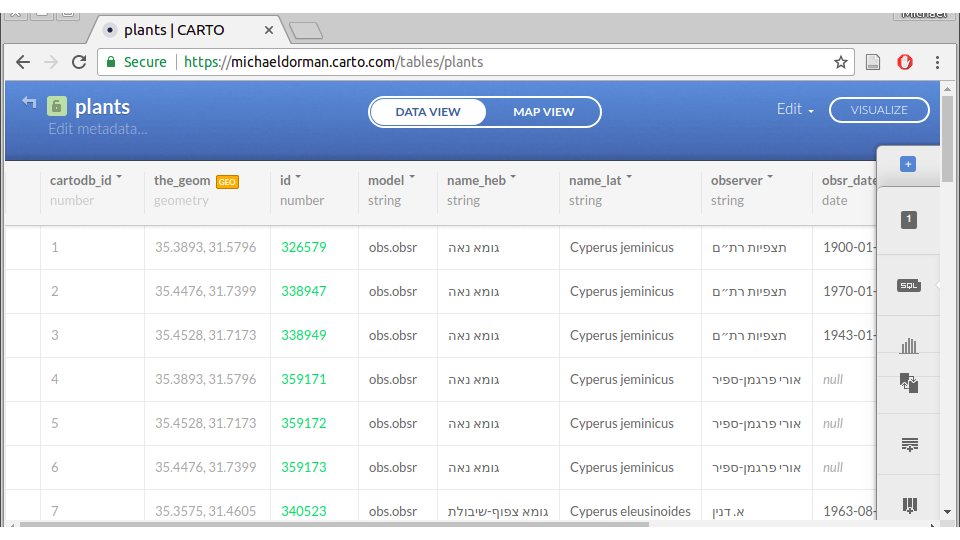
FIGURE 9.2: The plants table, as displayed in the CARTO web interface
Let’s try to send a query to the CARTO SQL API to get some data in the GeoJSON format from the plants table. Paste the following query into the browser’s address bar -
https://michaeldorman.carto.com/api/v2/sql?format=GeoJSON&q=
SELECT id, name_lat, the_geom FROM plants LIMIT 2
Since we chose GeoJSON as the format, a GeoJSON file will be returned. The query q was SELECT id, name_lat, the_geom FROM plants LIMIT 2, which means that we request the id, name_lat and the_geom columns from the plants table, limited to the first 2 records.
As a result, the CARTO server takes the relevant information from the plants table and returns the following GeoJSON content -
{
  "type": "FeatureCollection",
  "features": [
    {
      "type": "Feature",
      "geometry": {
        "type": "Point",
        "coordinates": [35.032018, 32.800539]
      },
      "properties": {
        "id": 345305,
        "name_lat": "Elymus elongatus"
      }
    },
    {
      "type": "Feature",
      "geometry": {
        "type": "Point",
        "coordinates": [35.564703, 33.047197]
      },
      "properties": {
        "id": 346805,
        "name_lat": "Galium chaetopodum"
      }
    }
  ]
}
This is a GeoJSON string of type FeatureCollection (Section 7.2.4). It contains two features with Point geometries, each having two non-spatial attributes id and name_lat.
Remember that the geometry column the_geom needs to appear whenever we request a spatial layer format such as GeoJSON, otherwise the server cannot generate the geometric part of the layer and we would get an error. For example, omitting the the_geom column from the above query -
https://michaeldorman.carto.com/api/v2/sql?format=GeoJSON&q=
SELECT id, name_lat FROM plants LIMIT 2
Returns the following error message instead of the requested GeoJSON -
{"error":["column \"the_geom\" does not exist"]}By the way, while pasting these URL examples into the browser, you may have noticed how the browser automatically encodes the URL into a format that can be transmitted over the Internet. This is something that happens automatically and we do not need to worry about.
For example, spaces are converted to %20, so that the URL we typed above -
https://michaeldorman.carto.com/api/v2/sql?format=GeoJSON&q=
SELECT * FROM plants LIMIT 2
Becomes -
https://michaeldorman.carto.com/api/v2/sql?format=GeoJSON&q=
SELECT%20id,%20name_lat,%20geom%20FROM%20plants%20LIMIT%202
Since the returned file is in the GeoJSON format, we can immediately import it into various spatial applications. For example, the file can be added as a layer and inspected in GIS software such as QGIS (Figure 9.3). If you are not using GIS software, you can still examine the GeoJSON file by importing it into the geojson.io web interface (Figure 7.2). More importantly to our cause, the GeoJSON content can be instantly loaded in a Leaflet web map, as will be demonstrated next in Section 9.8.
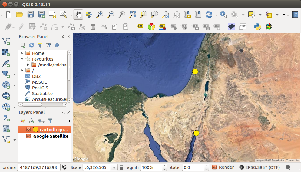
FIGURE 9.3: A GeoJSON file, obtained from the CARTO SQL API, displayed in QGIS
Exporting data in the JSON format is very similar to GeoJSON, but applicable for non-spatial queries that cannot be converted to GeoJSON. We will see a practical example of exporting JSON data from CARTO in Section 10.4.3.
- Try one of the above non-spatial SQL query examples with the CARTO SQL API, using the JSON as the export format
Lastly, as an example of the CSV export format try the following request to the SQL API -
https://michaeldorman.carto.com/api/v2/sql?format=CSV&q=
SELECT id, name_lat, obsr_date, ST_AsText(the_geom) AS geom
FROM plants WHERE name_lat = 'Iris mariae' LIMIT 3;
Note that we use the format=CSV parameter so that the result comes as a CSV file. CSV is a plain-text tabular format, in the present example containing the following text -
id,     name_lat,    obsr_date,  geom
358449, Iris mariae, 2010-03-13, POINT(34.412502 31.019879)
359806, Iris mariae, 2015-03-08, POINT(34.713009 30.972615)
337260, Iris mariae, 2001-02-23, POINT(34.63678 30.92807)
The CSV file can also be examined in a spreadsheet software such as Microsoft Excel or LibreOffice (Figure 9.4).
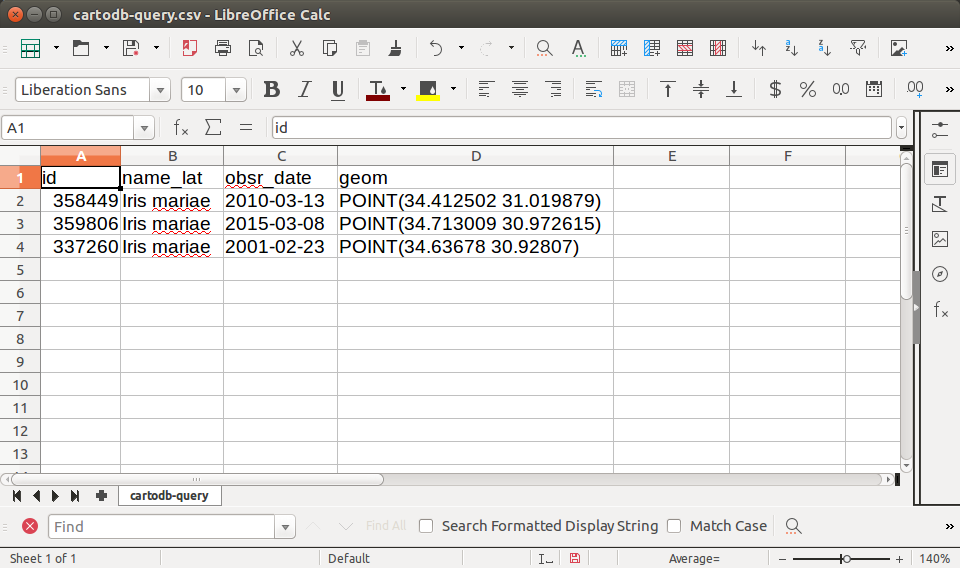
FIGURE 9.4: CSV file exported from the CARTO SQL API displayed in a spreadsheet sowtware (LibreOffice Calc)
For a more detailed discussion of the CARTO SQL API, also see the documentation as well as the above-mentioned SQL API Tutorial.
9.7.3 Uploading your data
Before we begin with connecting a Leaflet map with data from CARTO, you may want to experiment with your own account, possibly with different data instead of the plants table. Assuming you already signed up and have a CARTO account, the easiest way to upload data is the use the CARTO web interface.
Follow these steps to get your data on CARTO -
- Go to https://carto.com/ and login to your account
- Once you are in your user’s home page, click on Maps in the upper-left corner of the screen and then click on Your datasets in the dropdown menu. This screen shows the different tables in your database on CARTO. For example, Figure 9.5 shows the datasets page with two tables named
beer_shevaandearthquake_sql. This screen may be empty if created a new CARTO account and haven’t uploaded any data yet. - Click on the NEW DATASET button in the top-right corner of the screen
- You will see different buttons for various methods of importing data. The simplest option is to upload a GeoJSON file. Choose the Data file option in the upper ribbon, then click on the BROWSE button and navigate to your GeoJSON file. Finally, click on the CONNECT DATASET button (Figure 9.6). You can upload the
plants.geojsonfile from the book materials into your own account to experiment with the same dataset as shown in the examples. - Once the file is uploaded it is included as a new table in your CARTO database, and will appear in the list of your datasets. You can view the table in the CARTO web interface (Figure 9.2), and even edit its contents. For example, you can change the table name (in the top left corner in the table view), rename any of the columns, edit cell contents, add new rows, etc.
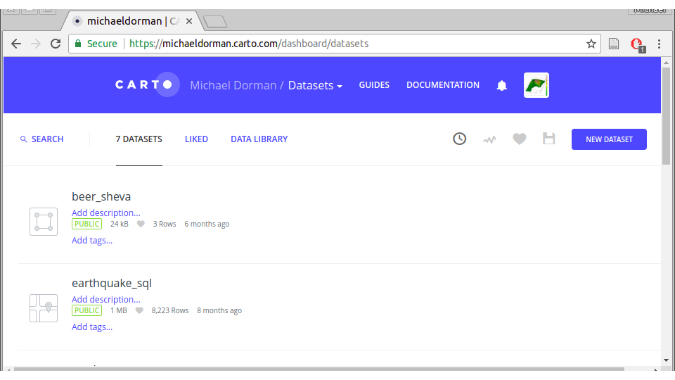
FIGURE 9.5: Datasets screen on CARTO
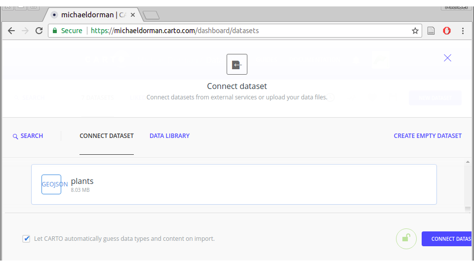
FIGURE 9.6: The file upload screen in the CARTO web interface
- Upload any GeoJSON file other than
plants.gejsonto CARTO, then try to adapt the above SQL API queries to your own username, table name and column names- Test the new queries by pasting them into the browser address bar and examining the returned content
9.8 CARTO and Leaflet
In the previous section, we learned how to use the CARTO SQL API to send SQL queries to a CARTO database. Importantly, since we are working with a spatial database, one of the formats in which we can choose to return our result is GeoJSON.
In this section, we will load the query result in a web page to display it on a Leaflet map. The method we are going to use is the $.getJSON function, which we introduced in Section 7.7 and used in numerous examples in the last two Chapters 7 and 8 for loading GeoJSON layers from files.
Our starting point is the basic map example-06-02.html from Chapter 6, with two small changes.
First, we include the jQuery library in the <head>, since we will use the $.getJSON function from that library -
<script src="js/jquery.js"></script>Second, we change the initial map extent as follows, so that the plants observations will be visible -
var map = L.map("map").setView([32, 35], 8);Now, in order to load data from CARTO on this map, we will perform the following steps -
- Construct the URL to query the CARTO SQL API
- Request the data from CARTO and add it on the map
In the first step, we will construct the query URL, which consists of the (fixed) base URL prefix and the variable SQL query suffix. Using the complete URL we will retrieve the data from the CARTO database.
The base URL, specific to our user name on CARTO, can be kept in a separate variable hereby named url so that we do not need to repeat in with each and every query we make in our <script> -
var url = "https://michaeldorman.carto.com/api/v2/sql?" +
    "format=GeoJSON&q=";
Note that to make the code even more manageable you can also split the base URL into two parts, keeping the user name in a separate variable. That way, when changing accounts it is more clear which part needs to be modified.
var cartoUserName = "michaeldorman";
var url = "https://" + cartoUserName +
    ".carto.com/api/v2/sql?format=GeoJSON&q=";
Either way, our next step is to define an SQL query used to retrieve data from the database. For example, we can use the following query which returns the name_lat and the_geom columns for the first 25 record from the plants table. Remember that you need to include the geometry column in your query whenever the requested format is GeoJSON, otherwise the layer cannot be generated and we will get an error.
var sqlQuery = "SELECT name_lat, the_geom FROM plants LIMIT 25";When the base URL and the SQL query are combined, using url+sqlQuery, we get the complete URL, as follows -
https://michaeldorman.carto.com/api/v2/sql?format=GeoJSON&q=
SELECT name_lat, the_geom FROM plants LIMIT 25
The complete URL can then be passed to $.getJSON to load the response from CARTO on a Leaflet map -
$.getJSON(url + sqlQuery, function(data) {
    L.geoJSON(data, {
        onEachFeature: function (feature, layer) {
            layer.bindPopup(feature.properties.name_lat);
        }
    }).addTo(map);
});
This code should be familiar from Chapters 7 and 8. The outermost function is $.getJSON, which we use to make an Ajax GET request from another location on the internet (CARTO, in this case).
Since the returned data are in the GeoJSON format (remember we used format=GeoJSON), the callback function of $.getJSON can use the L.geoJSON function to immediately convert the GeoJSON object to a Leaflet GeoJSON layer. Using the onEachFeature option we also bind specific popups (Section 8.5) for each feature to display the (Latin) name of the observed plants. Finally, the layer is added on the map with the .addTo method.
The complete code section we add at the bottom of the basic map <script>, for loading data from CARTO on our Leaflet map, is shown below -
var url = "https://michaeldorman.carto.com/api/v2/sql?" +
    "format=GeoJSON&q=";
var sqlQuery = "SELECT name_lat, the_geom FROM plants LIMIT 25";

$.getJSON(url + sqlQuery, function(data) {
    L.geoJSON(data, {
        onEachFeature: function (feature, layer) {
            layer.bindPopup(feature.properties.name_lat);
        }
    }).addTo(map);
});
The resulting map example-09-01.html is shown on Figure 9.7. Our data from CARTO, i.e. the first 25 plant observations, are loaded on the map!
FIGURE 9.7: example-09-01.html (Click to view this example on its own)
- Paste the above code section into the console of
example-09-01.html- Modify the SQL query (
sqlQuery) to experiment with adding different observations on the map, according to the SQL examples shown in Section 9.6- For example, you can replace the
LIMIT 25part with a condition of the formWHERE name_lat = '...'to load all observations of a certain species
We have just seen the general principle of using the CARTO SQL API to display layers coming from a database on a Leaflet map. So far, what we did was not very different than loading a GeoJSON file on a map, much like in the examples from Chapters 7 and 8. The only difference is that the path to the GeoJSON file was given as a URL addressing the CARTO SQL API, rather than a local (Section 7.7.2) or remote (Section 7.7.3) static file. Still, the query was constant, so that the same 25 observations are loaded each time the page is opened (unless the database itself is modified).
In the beginning of the Chapter we mentioned that one of the main reasons of using a database in web mapping is that we can display subsets of the data, selected according to user input. That way, we can have large amounts of data “behind” the web map, while maintaining responsiveness due to the fact that small portions of the data are transferred to the client each time. To fully exploit the advantages of connecting a database to a web map, in the next two Chapters we will see examples where the SQL query is generated dynamically, in response to user input -
9.9 Exercise
- The following SQL query returns the (sorted) species list from the
plantstable of rare plants -SELECT DISTINCT name_lat FROM plants ORDER BY name_lat- Load the result of the query inside a web page, and use it to dynamically generate an unordered list (
<ul>) of all unique plant species names in the database (Figure 9.8)- Remember that the query is not spatial (i.e. it does not contain the geometry column), so you need to use
format=JSONinstead offormat=GeoJSONto get the result in the JSON format- You can use
example-04-08.htmlfrom Section 4.12 (Figure 4.9), where we have generated an unordered list based on an array, as a starting point
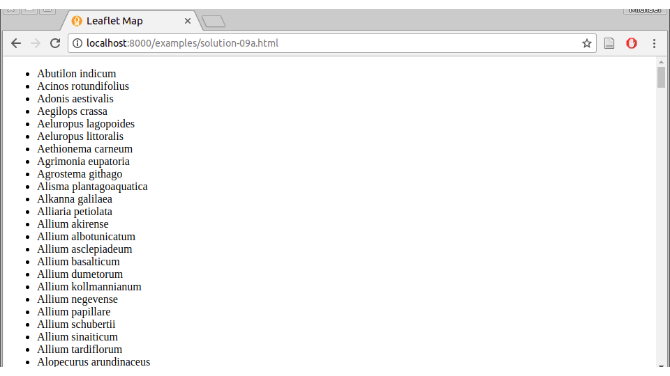
FIGURE 9.8: solution-09.html
References
Obe, R, and L Hsu. 2015. PostGIS in Action. 2nd ed. Manning Publications Co., USA. http://www.postgis.us/.