Chapter 11 Spatial queries
Last updated: 2018-11-11 20:44:59
11.1 Introduction
In this Chapter, we are going to integrate our web map with spatial SQL queries to selectively load data from the CARTO database, based on geographical distance. Specifically, we will build a web map where the user can click on any location, and as a result the nearest n plant locations to the clicked location are loaded from the database and displayed, along with straight-line paths towards those plants. You can see the final result on Figure 11.8.
We will build this web map with several steps, each time adding further functionality -
- Adding a marker at the clicked location on the map (Section 11.2.1)
- Adding a custom marker at clicked location, to distinguish from the observation markers (Section 11.2.2)
- Finding n nearest observations, using a spatial SQL query, and adding them on the map (Section 11.4)
- Drawing line segments from clicked location to the nearest observations (Section 11.5)
11.2 Adding marker on click
11.2.1 Getting click coordinates
Our first step towards a web map that queries the plants table based on spatial proximity is to mark the clicked location on the map and capture its coordinates. The coordinates will be stored to pass them on with a spatial SQL query (Section 9.6.4). We start from our basic map (example-06-02.html) from Section 6.5 and make changes on top of it. First, we will modify the initially displayed map extent to a larger one -
var map = L.map("map").setView([32, 35], 8);Next, we will add a layer group named myLocation. This layer will contain the clicked location marker, created on map click. As we have seen in Sections 7.5.3 and 10.5.3, using a layer group will make it easy to remove the old marker before adding a new one, in case when the user changed his/her mind and clicks on a different location.
var myLocation = L.layerGroup().addTo(map);We then define an event listener, which will execute a function named mapClick each time the user clicks on the map. Remember the map click event and its .latlng property introduced in the example-06-08.html from Section 6.9? We use the same principle here, only that instead of adding a popup with the clicked coordinates in the clicked location, we are adding a marker.
First, we set the event listener for "click" events on the map object, referencing the mapClick function we have yet to define -
map.on("click", mapClick);Second, we need to define the mapClick function itself. The mapClick function does two things -
- Clearing the
myLocationlayer of any previous markers (from a previously clicked location, if any) - Adding a new marker to the
myLocationlayer, at the clicked coordinates using the.latlngproperty of the event object
Here is the code for the mapClick function -
function mapClick(e) {
    myLocation.clearLayers();
    L.marker(e.latlng).addTo(myLocation);
}
As a result, we now have a map (example-11-01.html) where the user can click, with the last clicked location displayed marked on the map (Figure 11.1).
FIGURE 11.1: example-11-01.html (Click to view this example on its own)
11.2.2 Adding custom marker
Shortly, we will write code to load plant observation nearby to our clicked locations, and display them as markers too. To distinguish the marker for the clicked location from the markers for the plant observations we need to override the default blue marker settings in Leaflet and display a different type of marker for one of the two layers. For example, we can draw a red marker for the clicked location, and keep the blue markers denoting the plant locations (Figure 11.7). To change marker settings, we first need to understand a little better how the marker appearance is defined in the first place.
The markers we see on a Leaflet map, created with L.marker (Section 6.6.1), are in fact PNG images displayed at the specified locations placed on top of the map background. If you look closely, you will see that the default blue marker also has a “shadow” effect behind it, to create an illusion of 3D, i.e. the marker “sticking out” of the map (Figure 11.2). The shadow is a PNG image too, displayed behind the PNG image of the marker itself. We can use the “inspect” pane in the Developer Tools to figure out which PNG image is actually being loaded by Leaflet, and where does it come from (Figure 11.3). Doing so reveals the following values for the src attributes of the <img> elements for the marker and marker shadow images -
- https://unpkg.com/leaflet@1.3.1/dist/images/marker-icon.png
- https://unpkg.com/leaflet@1.3.1/dist/images/marker-shadow.png
FIGURE 11.2: Deafult and custom images for drawing a Leaflet marker
FIGURE 11.3: Inspecting Leaflet icon element
You can follow these URLs to download and inspect the PNG images in any graphical viewer or editor (such as “Microsoft Paint”).
To distinguish our clicked location from other markers on the map we will use a different marker for the clicked location. In our example, we will use a marker PNG image which is the same as the default one, only colored in red instead of the default blue color (Figure 11.2). The PNG images for the red icon are stored in the online book materials (Appendix A) -
To set a custom Leaflet marker type based on these PNG images, you need to place the files on your server. For example, the files can be placed in a folder named images within the root directory of the web page (see Section 5.5.2). A custom marker using these PNG images, assuming they are in the images folder, is then defined with the L.icon function as follows -
var redIcon = L.icon({
    iconUrl: "images/redIcon.png",
    shadowUrl: "images/marker-shadow.png",
    iconAnchor: [12, 41]
});
The L.icon function requires a path to the PNG images for the icon iconUrl, and (optionally) a path to the PNG image for the shadow shadowUrl. The other important parameter is iconAnchor, which sets the anchor point, i.e. the exact icon image pixel which corresponds to the point coordinates where the marker is initiated. The custom icon object is assigned to a variable, hereby named redIcon, which we can later use to draw custom markers on the map with L.marker.
What is the meaning of iconAnchor, and why did we use the value of [12, 41]? The iconAnchor parameter specifies which pixel on the marker will be placed on the [lon, lat] point where the marker is placed. To determine the right anchor point coordinates, we need to figure out the size (in pixels) of our particular marker, and the image region where we would like the anchor to be placed in. The image size can be determined by viewing the PNG file properties, for example clicking on the file with the right mouse button, choosing Properties and then the Details tab. In our case, the size of the redIcon.png image is 25 by 41 pixels (Figure 11.4).
FIGURE 11.4: File properties for the red icon redIcon.png. The highlighted entry shows image dimensions in pixels (25 x 41)
Conventionally, image coordinates are set from a [0, 0] point at the upper left corner of the icon. The anchor point for our particular icon should be at its tip, at the middle-bottom. Starting from the top-left corner [0, 0], this means going all the way down on the Y-axis, then half-way to the right on the X-axis. Since the PNG image size is [25, 41], this means we set the the pixel on the center of the X-axis [12, ...] and bottom of the Y-axis [..., 41], thus the anchor value of [12, 41] (Figure 11.5).
FIGURE 11.5: PNG image for the red marker redIcon.png, with coordinates of the four corners and the coordinate of the marker anchor point. Note that the coordinate system starts from the top-left corner, with reversed Y-axis direction
Now that the redIcon object is ready and PNG images are in place, we can replace the last expression for adding a marker inside the map click event listener in example-11-01.html -
L.marker(e.latlng).addTo(myLocation);With a new expression that loads our custom redIcon marker in example-11-02.html -
L.marker(e.latlng, {icon: redIcon}).addTo(myLocation);You can use just about any PNG image as a marker icon this way, not just a differently colored default marker. There are many resources for getting prepared PNG images suitable for map markers, such as the Map Icons section on the https://www.flaticon.com website.
The resulting map (example-11-02.html) is shown on Figure 11.6. Clicking on the map now adds the red marker icon instead of the default blue one.
FIGURE 11.6: example-11-02.html (Click to view this example on its own)
- Download one of the PNG images for custom map icons from https://www.flaticon.com
- Adapt
example-11-02.htmlto display the icon you downloaded instead of the red icon
For other examples of using custom icons in Leaflet, check out the Leaflet Custom Markers Tutorial and the DUSPviz Map Design Tutorial.
11.3 Spatial PostGIS operators
11.3.1 Overview
Now that we know how to add a custom red marker on map click, we are going to add some code into our mapClick function incorporating a spatial SQL query (Section 9.6.4) to find the closest plants to the clicked location. As a result (Figure 11.7), each time the user clicks on a new point and mapClick adds a red marker, the function also queries for the nearest plants and display them on the map. In this Section (11.3), we will discuss the structure of the required spatial SQL query to return nearest features. Then, in Section 11.4, we will see how to implement this type of SQL query in our Leaflet map.
As we have already discussed in Section 9.6.4, spatial databases are characterized by the fact that their tables may contain a geometry column. On CARTO, the geometry column is conventionally named the_geom (Section 9.7.2). The geometry column is composed of encoded geometric data in the WKB format, which can be used to transform returned table records to spatial formats such as GeoJSON. For example, in Chapters 9 and 10 we used SELECT statements to return GeoJSON objects based on data from the plants table on CARTO. This type of queries utilizes the the_geom geometry column to create the geomerty part of the GeoJSON. However, the geometry column can also be used to make various spatial calculations on our data, using spatial SQL operators and functions. A very common example of such a calculation is geographical distance.
11.3.2 Geographical distance
To find the five plant observations nearest to our clicked location, we can use the following query which was already given in Section 9.6.4 as an example of a spatial SQL query -
SELECT name_lat, obsr_date, ST_AsText(the_geom) AS geom
  FROM plants
  ORDER BY
    the_geom::geography <->
    ST_SetSRID(
      ST_MakePoint(34.810696, 31.895923), 4326
    )::geography
  LIMIT 5;
This query returns the nearest five observations from the plants table, based on distance to a specific point [34.810696, 31.895923].
In this section, we will explain the structure of this query more in depth.
First of all, as we already saw in Chapters 9 and 10, limiting the returned table to the first n records can be triggered using the term LIMIT n, as in LIMIT 5 or LIMIT 25. However, we need the five nearest plants, not just the five plants incidentally being first in terms of the table row ordering. This means the data need to be ordered before being returned. As an example of non-spatial ordering, the table can be ordered with ORDER BY followed by column name(s) to select the five plant observations with the lowest (or highest) values for the given variable(s). For example, the following query returns the five earliest plant observation records. The ORDER BY obsr_date part means the table is ordered based on the values in the obsr_date (observation date) column -
SELECT name_lat, obsr_date, ST_AsText(the_geom) AS geom
  FROM plants
  ORDER BY obsr_date
  LIMIT 5;
Which gives the following result -
    name_lat    | obsr_date  |            geom
----------------+------------+----------------------------
 Iris haynei    | 1900-01-01 | POINT(35.654005 32.741372)
 Iris atrofusca | 1900-01-01 | POINT(35.193367 31.44711)
 Iris atrofusca | 1900-01-01 | POINT(35.189142 31.514754)
 Iris vartanii  | 1900-01-01 | POINT(35.139696 31.474149)
 Iris haynei    | 1900-01-01 | POINT(35.679761 32.770133)
(5 rows)
Try the corresponding CARTO SQL API query, choosing the CSV output format, to examine the above result on your own -
https://michaeldorman.carto.com/api/v2/sql?format=CSV&q=
SELECT name_lat, obsr_date, ST_AsText(the_geom) AS geom
FROM plants ORDER BY obsr_date LIMIT 5
Indeed, all returned records are from the 1900-01-01 which is the earliest date in the obsr_date field. Spatial ordering is similar, only that we have the table records ordered based on their spatial arrangement, namely based on their distances to another spatial feature or set of features. In other words, with spatial ordering, instead of ordering by non-spatial column values, we are ordering by distances which are calculated using the geometry column.
In the above spatial query for getting the five nearest points from a given location [34.810696, 31.895923], the only part different from the previous non-spatial query is basically the ORDER BY term.
Instead of the following ORDER BY term for non-spatial ordering, based on obsr_date values -
ORDER BY obsr_dateWe have the following ORDER BY term, for spatial ordering, based on distance from a specific point [34.810696, 31.895923] -
ORDER BY
  the_geom::geography <->
  ST_SetSRID(ST_MakePoint(34.810696, 31.895923), 4326)::geography
The result is as follows -
       name_lat       | obsr_date  |            geom
----------------------+------------+----------------------------
 Lavandula stoechas   | 1931-04-30 | POINT(34.808564 31.897377)
 Bunium ferulaceum    |            | POINT(34.808504 31.897328)
 Bunium ferulaceum    | 1930-02-23 | POINT(34.808504 31.897328)
 Silene modesta       | 1900-01-01 | POINT(34.822295 31.900125)
 Corrigiola litoralis | 2016-01-30 | POINT(34.825931 31.900792)
(5 rows)
These are the locations and some properties of the five nearest plants to the specified location. You can see that the longitude and latitude values are fairly similar to [34.810696, 31.895923], reflecting the fact that the points are proximate.
Again, you can experiment with this query in the CARTO SQL API -
https://michaeldorman.carto.com/api/v2/sql?format=CSV&q=
SELECT name_lat, obsr_date, ST_AsText(the_geom) AS geom
FROM plants
ORDER BY the_geom::geography <-> ST_SetSRID(
ST_MakePoint(34.810696, 31.895923), 4326)::geography LIMIT 5;
As you probably noticed, the expression used for spatial ordering is more complicated than simply a column name such as obsr_date.
the_geom::geography <->
ST_SetSRID(ST_MakePoint(34.810696, 31.895923), 4326)::geography
In addition to the column name the_geom, this particular ORDER BY term contains four spatial PostGIS functions and operations which we will now explain -
ST_MakePointST_SetSRID::geography<->
A two-dimensional point geometry is constructed using the ST_MakePoint function, given two coordinates x and y, in this case 34.810696 and 31.895923, respectively. Thus, the expression ST_MakePoint(34.810696, 31.895923) defines a single geometry of type "Point", which we can use in spatial calculations.
The ST_SetSRID function then sets the coordinate reference system (CRS) for the geometry. The 4326 argument is the EPSG code of the WGS84 geographical projection (i.e. lon/lat) (Figure 6.1).
The ::geography part determines that what follows is a calculation with spherical geometry, which is the appropriate way to do distance-based calculations with lon/lat data. With ::geography, distance calculations give the spherical Great Circle distance, in meters. Omitting the ::geography part is equivalent to using the default ::geometry, implying that what follows is a planar geometry calculation. Planar geometry calculations are only appropriate for projected data, which we do not use in this book. In the case of non-projected lon/lat data, using ::geometry gives straight-line euclidean distance in degree units, which is almost always inappropriate.
The <-> operator returns the 2D distance between two sets of geometries. Since we set ::geography, the result represents spherical Great Circle distance in meters. In this case, we are calculating the distances between the_geom, which is the geometry column of the plants layer, and an individual point. The result is a series of distances in meters, corresponding to all features of the plants table.
Finally, the series of distances is passed to the ORDER BY keyword, thus rearranging the table based on the calculated distances, from the smallest to largest, i.e. nearest observation to furthest. The LIMIT 5 part then takes the top five records, which are the five nearest ones to [34.810696, 31.895923].
11.3.3 Sphere vs. Shperoid
As another demonstration of the four spatial PostGIS functions discussed in Section 11.3.2 above, consider the following small query. This query calculates the distance between two points [0, 0] and [0, 1] in geographic coordinates (lon/lat), i.e. the length of one degree of longitude along the equator -
SELECT
  (ST_SetSRID(ST_MakePoint(0, 0), 4326)::geography <->
  ST_SetSRID(ST_MakePoint(1, 0), 4326)::geography) / 1000
AS dist_km;
The result gives the distance of 111.195 km -
     dist_km
------------------
 111.195079734632
(1 row)
Note that, in this case, we are manually constructing two points in WGS84, [0, 0] and [1, 0], using ST_MakePoint, ST_SetSRID and ::geography. The 2D distance operator <-> is the applied on the points to calculate the Great Circle distance between them, in meters. Dividing the result by 1000 transforms it from meters to kilometers.
The true distance between [0, 0] and [1, 0], however, is 111.320 km and not 111.195. What is the reason for the discrepancy? The reason is that the <-> operator, though using spherical geometry, relies on a sphere model of the earth, rather than the more accurate spheroid model. In PostGIS, the more accurate but somewhat slower distance calculation based on a spheroid can be obtained with ST_Distance instead of <->, as in -
SELECT ST_distance(
  ST_SetSRID(ST_MakePoint(0, 0), 4326)::geography,
  ST_SetSRID(ST_MakePoint(1, 0), 4326)::geography) / 1000
AS dist_km;
Giving the more accurate result of 111.319 km-
     dist_km
-----------------
 111.31949079327
(1 row)
Though ST_distance gives the more accurate estimate, the calculation takes longer. For example, finding the 5 nearest neighbors from the plants table takes 170.967 ms using the <-> operator, compared to 370.637 ms with ST_Distance. This is more than twice longer calculation time. In this example, exactly the same five plants are chosen in both cases, but it is possible for the ordering to be incorrect in some cases, due to the small difference in distance estimates between the sphere and spheroid methods. In practice, the trade-off between speed and accuracy should always be considered when choosing the right distance-based calculation given the application requirements, dataset resolution and dataset size. With small amounts of data and/or high accuracy requirements ST_Distance should be preferred; otherwise the accuracy given by <-> may be sufficient.
- What do you think will happen if we omit the
::geographykeyword from both places where it appears in the above query?- Check your answer using the CARTO SQL API
The above is just a glimpse of spatial operators in PostGIS, which is a large topic to cover. A good introduction to spatial operators in PostGIS, also using the CARTO platform, can be found in the series of tutorials by CARTO -
11.4 Adding nearest points to map
We can use the above SQL spatial query in the mapClick function, so that the nearest 25 plants are displayed along with the red marker. The key here is that we are going to make the spatial query dynamic, each time replacing the ordering according to location chosen by the user on the web map. Unlike in the above example, where the longitude and latitude were hard-coded into the SQL query (as in [34.810696, 31.895923]), we are going to generate the SQL query by pasting user-clicked coordinates into the SQL query “template”. Specifically, we will use longitude and latitude returned from our click event and stored in the myLocation variable (Section 11.2.1).
We proceed, modifying example-11-02.html. First, we add two more variable definitions: a layer for the nearest plant markers plantLocations, and the URL for querying the CARTO SQL API url. Along with the marker layer which was already defined in the previous example myLocation, the variable definition part in our <script> is now composed of the following three expressions -
var myLocation = L.layerGroup().addTo(map);
var plantLocations = L.layerGroup().addTo(map);
var url = "https://michaeldorman.carto.com/api/v2/sql?" +
    "format=GeoJSON&q=";
The remaining required changes are additions inside our mapClick function. In its new version, the function will not only display the clicked location, but also the locations of 25 nearest observations of rare plants.
To remind, the previous version of the mapClick function in example-11-02.html (Section 11.2.1) merely cleared the old marker and added a new one according to the e.latlng object -
function mapClick(e) {
    myLocation.clearLayers();
    L.marker(e.latlng, {icon: redIcon}).addTo(myLocation);
}
In the new version of the function, we add four new expressions.
First, we define a new local variable clickCoords capturing the contents of e.latlng for that particular event. This is just a convenience, for typing clickCoords rather than e.latlng in the various places where we will use the clicked coordinates in the function code body.
var clickCoords = e.latlng;Second, we make sure that the nearest plant observations are cleared between consecutive clicks, just like the red marker is. The following expression takes care of clearing the previously loaded plantLocations contents -
plantLocations.clearLayers();In the third expression, we dynamically compose the SQL query string to get 25 nearest records from the plants table considering the clicked location. We basically replace the hard-coded lon/lat coordinates from the spatial ordering SQL query discussed in Section 11.3.2 with the lng and lat properties of the clickCoords object defined above. The result, named sqlQueryClosest, will now contain the specific SQL query string needed to obtain the 25 nearest plants from our currently clicked location. This is conceptually similar to the way that we dynamically constructed an SQL query to select the observations of a particular species in Section 10.5.3.
var sqlQueryClosest =
    "SELECT name_lat, the_geom FROM plants" +
    "ORDER BY the_geom::geography <->" +
    "ST_SetSRID(ST_MakePoint(" +
    clickCoords.lng + "," + clickCoords.lat +
    "), 4326)::geography LIMIT 25";
Fourth, we use the sqlQueryClosest string to request the nearest 25 observations from CARTO, and add them to the plantLocations layer. The popup, in this case, contains the Latin species name name_lat displayed in italics.
$.getJSON(url + sqlQueryClosest, function(data) {
    L.geoJSON(data, {
        onEachFeature: function(feature, layer) {
            layer.bindPopup(
                "<i>" + feature.properties.name_lat + "</i>"
            );
        }
    }).addTo(plantLocations);
});
Here is the complete code for the new version of the mapClick function -
function mapClick(e) {

    // Get clicked coordinates
    var clickCoords = e.latlng;

    // Clear map
    myLocation.clearLayers();
    plantLocations.clearLayers();

    // Add location marker
    L.marker(clickCoords, {icon: redIcon}).addTo(myLocation);

    // Set SQL query
    var sqlQueryClosest =
        "SELECT name_lat, the_geom FROM plants" +
        "ORDER BY the_geom::geography <->" +
        "ST_SetSRID(ST_MakePoint(" +
        clickCoords.lng + "," + clickCoords.lat +
        "), 4326)::geography LIMIT 25";

    // Get GeoJSON & add to map
    $.getJSON(url + sqlQueryClosest, function(data) {
        L.geoJSON(data, {
            onEachFeature: function(feature, layer) {
                layer.bindPopup(
                    "<i>" + feature.properties.name_lat + "</i>"
                );
            }
        }).addTo(plantLocations);
    });

}
The resulting map (example-11-03.html) is shown on Figure 11.7.
FIGURE 11.7: example-11-03.html (Click to view this example on its own)
11.5 Drawing line connectors
To highlight the direction and distance from the clicked location to each of the queried plants, the final version example-11-04.html adds code for drawing line segments between the focal point and each observation. This is a common visualization technique, also known as a “spider diagram” or “desire Line” (e.g. in ArcGIS help). It is frequently used to highlight the association between a focal point or points, and their associated (usually nearest) surrounding points from a different layer. For example, the lines can be used to visualize the association between a set of business stores and the customers who are potentially affiliated with each store.
To draw each of the line segments connecting the red marker (clicked location) with one of the blue ones (plant observation), we can take the two pairs of coordinates and apply the L.polyline function on them. The principle is similar to the function we wrote in the exercise for Chapter 3 (Section 3.11). Suppose that the clicked location coordinates are [lon0, lat0] and the coordinates of the first nearest plant are [lon1, lat1], [lon2, lat2], [lon3, lat3], etc. The coordinate arrays of the corresponding line segments, connecting each pair of points, are then -
[[lon0, lat0], [lon1, lat1]]for the first segment[[lon0, lat0], [lon2, lat2]]for the second segment[[lon0, lat0], [lon3, lat3]]for the third segment- etc.
Each of these coordinate arrays can be passed to the L.polyline function to draw the corresponding segment connecting a pair of points, much like the line segment connecting Building 72 with the Library (Section 6.6.2). Note that we will actually be using revered coordinate pairs, such as [lat0, lon0], as expected by all Leaflet functions for drawing shapes including L.polyline (Section 6.5.4).
To implement the above procedure of drawing line segments, we first create yet another layer group named lines at the beginning of our script, right below the expressions where we already defined myLocation and plantLocations layer groups -
var lines = L.layerGroup().addTo(map);Accordingly, inside the mapClick function we clear all previous line segments before new ones are drawn, with the following expression clearing the lines contents, right below the expressions where we clear mylocation and plantLocations -
lines.clearLayers();Moving on to the actual segment drawing. Inside the L.geoJSON function call, rather than just binding the Latin species name popup like we did in the previous example -
L.geoJSON(data, {
    onEachFeature: function(feature, layer) {

        // Bind popup
        layer.bindPopup(
            "<i>" + feature.properties.name_lat + "<i>"
        );

    }
}).addTo(plantLocations);
We add three more expressions inside the onEachFeature option. The expressions are used to draw a line segment between the “central” point where the red marker is, which is stored in clickCoords, and the currently added GeoJSON point, which is given in feature as part of the onEachFeature iteration (Section 8.5).
L.geoJSON(data, {
    onEachFeature: function(feature, layer) {

        // Bind popup
        layer.bindPopup(
            "<i>" + feature.properties.name_lat + "<i>"
        );

        // Draw line segment
        var layerCoords = feature.geometry.coordinates;
        var lineCoords = [
            [clickCoords.lat, clickCoords.lng],
            [layerCoords[1], layerCoords[0]]
        ];
        L.polyline(
            lineCoords,
            {color: "red", weight: 3, opacity: 0.75}
        ).addTo(lines);

    }
}).addTo(plantLocations);
The new code section, right below the //Draw line segment comment, is composed of three expressions, which we now discuss step by step.
In the first expression, we extract the coordinates of the current plant observation and assign it in a local variable named layerCoords -
var layerCoords = feature.geometry.coordinates;As discussed in Section 8.5, as part of the onEachFeature iteration, the currently processed GeoJSON feature is accessible through the feature parameter. Just like we are accessing the current species name with feature.properties.name_lat to include it in the popup, we can also extract the point coordinates with feature.geometry.coordinates. The feature.geometry.coordinates property of a GeoJSON "Point" geometry is an array of the form [lon, lat] (Section 7.2.2.2), which we store in a variable named layerCoords.
In the second expression, we build the segment coordinates array by combining the coordinates of the focal point stored in clickCoords with the coordinates of the current plant observation stored in layerCoords. Note that while layerCoords are stored as [lon, lat] according to the GeoJSON specification, L.polyline expects [lat, lon]. This is why the coordinates order is reversed with [layerCoords[1], layerCoords[0]].
var lineCoords = [
    [clickCoords.lat, clickCoords.lng],
    [layerCoords[1], layerCoords[0]]
];
The complete coordinates array is assigned into a variable named lineCoords.
In the third expressions, lineCoords is passed to the L.polyline function to create a line layer object. The .addTo method is then applied, in order to add the segment to the lines layer and thus actually draw it on the map.
L.polyline(
    lineCoords,
    {color: "red", weight: 3, opacity: 0.75}
).addTo(lines);
The resulting map (example-11-04.html) is shown on Figure 11.8. Try clicking on the map now displays both nearest plant observations and the connecting line segments.
FIGURE 11.8: example-11-04.html (Click to view this example on its own)
11.6 Exercise
Start with example-11-04.html and modify the code so that the popup for each of the nearest plants also specifies its distance to the queried point (Figure 11.9).
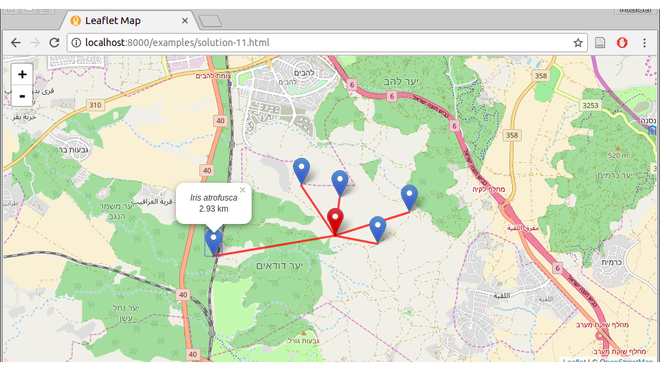
FIGURE 11.9: solution-11.html
To get the distances, you can use the following SQL query example which returns the five nearest plants along with the distance in kilometers to the specific point [34.810696, 31.895923]. The distances are given inside a column named dist_km.
SELECT name_lat,
  (
    the_geom::geography <->
    ST_SetSRID(
      ST_MakePoint(34.810696, 31.895923), 4326
    )::geography
  ) / 1000 AS dist_km,
  ST_AsText(the_geom) AS geom
FROM plants
ORDER BY dist_km
LIMIT 5;
This particular query gives the following result. Note the dist_km column, which contains the distances in kilometers.
       name_lat       |      dist_km      |            geom
----------------------+-------------------+----------------------------
 Lavandula stoechas   | 0.258166195505697 | POINT(34.808564 31.897377)
 Bunium ferulaceum    |  0.25928724896688 | POINT(34.808504 31.897328)
 Bunium ferulaceum    |  0.25928724896688 | POINT(34.808504 31.897328)
 Silene modesta       |  1.19050813583538 | POINT(34.822295 31.900125)
 Corrigiola litoralis |  1.53676126266166 | POINT(34.825931 31.900792)
(5 rows)
Here is the analogous CARTO SQL API query you can experiment with -
https://michaeldorman.carto.com/api/v2/sql?format=CSV&q=
SELECT name_lat, (the_geom::geography <->
ST_SetSRID(ST_MakePoint(34.810696, 31.895923), 4326
)::geography) / 1000 AS dist_km, ST_AsText(the_geom) as geom
FROM plants ORDER BY dist_km LIMIT 5
Remember that in the actual code you need to use format=GeoJSON instead of format=CSV, and the_geom instead of ST_AsText(the_geom) to get GeoJSON rather than CSV. It is also useful to round the distance values before putting them into the popup (e.g. to two decimal places, as shown on Figure 11.9). This can be done with JavaScript, applying the .toFixed method with the required number of digits on the numeric variable.
x = 2.321342;
x.toFixed(2); // Returns "2.32"