Chapter 8 Geometric operations with vector layers
Last updated: 2020-08-12 00:37:45
Aims
Our aims in this chapter are:
- Join by location and by attributes
- Make geometric calculations between vector layers
We will use the following R packages:
sfunits
8.1 Join by location
For most of the examples in this Chapter, we are going to use the US counties and three airports layers (Section 7.7.1):
library(sf)
airports = st_read("airports.geojson", stringsAsFactors = FALSE)
county = st_read("USA_2_GADM_fips.shp", stringsAsFactors = FALSE)
and transform them to the US National Atlas projection (Section 7.10):
Join by spatial location, or spatial join, is one of the most common operations in spatial analysis. In a spatial join we are “attaching” attributes from one layer to another based on their spatial relations. In ArcGIS this is done using “Join data from another layer based on spatial location” Figures 8.1–8.2.
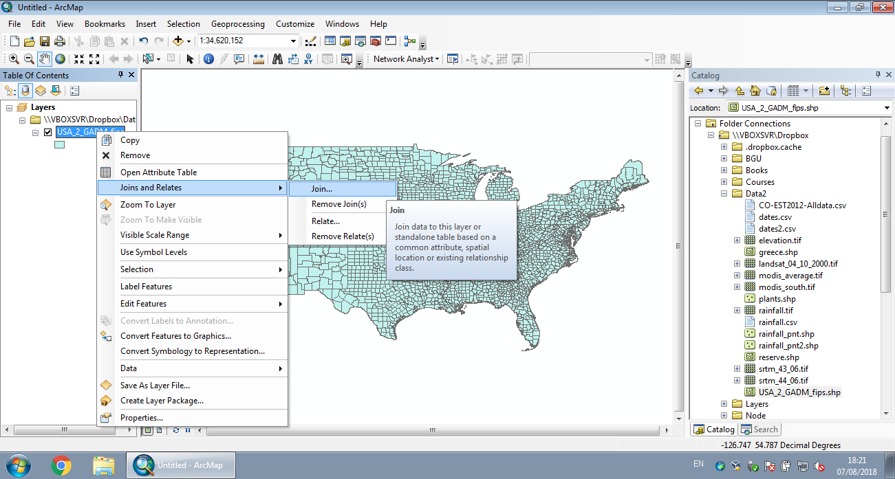
Figure 8.1: Join by location in ArcGIS (Step 1)
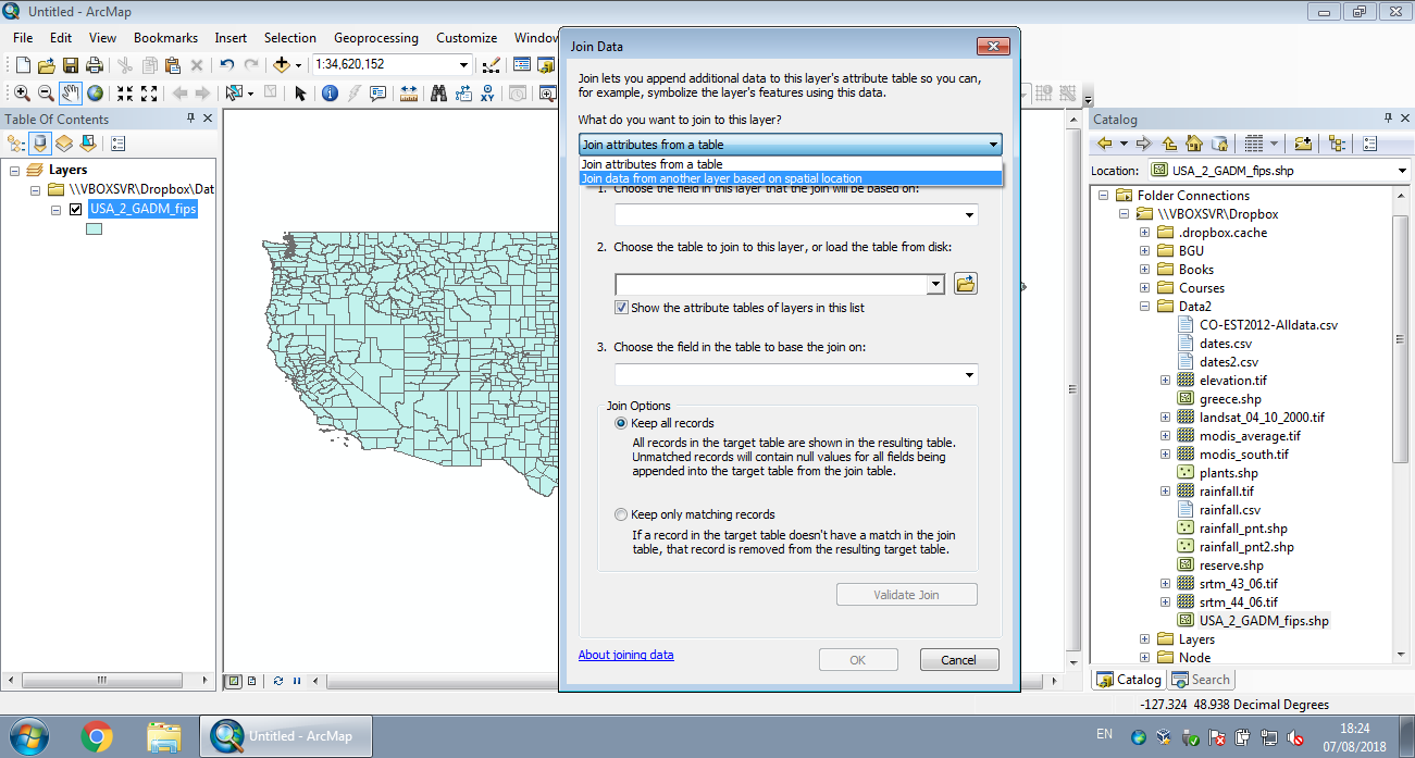
Figure 8.2: Join by location in ArcGIS (Step 2)
For simplicity, we will create a subset of the counties of New Mexico only, since all three airports are located in that state:
Figure 8.3 shows the geometry of the nm and airports layers:
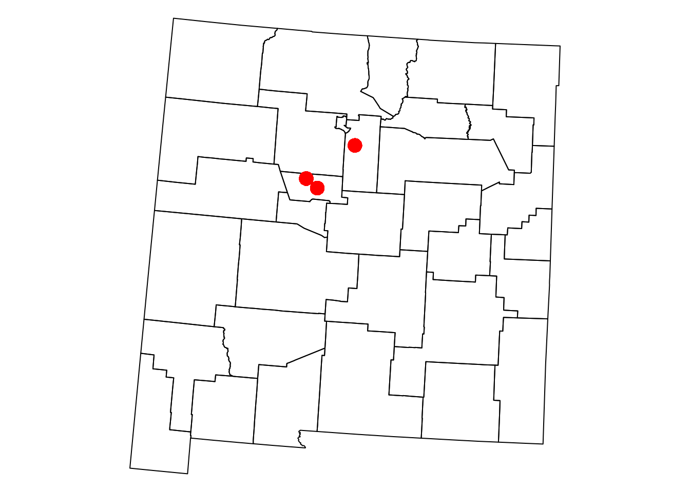
Figure 8.3: The nm and airports layers
Note that the pch parameter determines point shape (see ?points), while cex determines point size.
Given two layers x and y, a function call of the form st_join(x, y) returns the x layer along with matching attributes from y. The default join type is by intersection, other options can be specified using the join parameter (see ?st_join).
For example, the following expression joins the airports layer with the matching nm attributes. The resulting layer contains all three airports with their original geometry and name attribute, plus the NAME_1, NAME_2, TYPE_2 and FIPS of the nm feature that each airport intersects with:
st_join(airports, nm)
## Simple feature collection with 3 features and 5 fields
## geometry type:  POINT
## dimension:      XY
## bbox:           xmin: -619184.5 ymin: -1081605 xmax: -551689.8 ymax: -1022366
## projected CRS:  US National Atlas Equal Area
##                        name     NAME_1     NAME_2 TYPE_2  FIPS
## 1 Albuquerque International New Mexico Bernalillo County 35001
## 2           Double Eagle II New Mexico Bernalillo County 35001
## 3        Santa Fe Municipal New Mexico   Santa Fe County 35049
##                     geometry
## 1 POINT (-603868.2 -1081605)
## 2 POINT (-619184.5 -1068431)
## 3 POINT (-551689.8 -1022366)
What do you think will happen if we reverse the order of the arguments, as in
st_join(nm, airports)? How many features is the result going to have, and why?
8.2 Subsetting by location
We can create subsets based on intersection with another layer using the [ operator. An expression of the form x[y, ]—where x and y are vector layers—returns a subset of x features that intersect with y.
For example, the following expression returns only those nm counties that intersect with the airports layer:
The subset is shown in light blue in Figure 8.4:
plot(st_geometry(nm))
plot(st_geometry(nm1), col = "lightblue", add = TRUE)
plot(st_geometry(airports), col = "red", pch = 16, cex = 2, add = TRUE)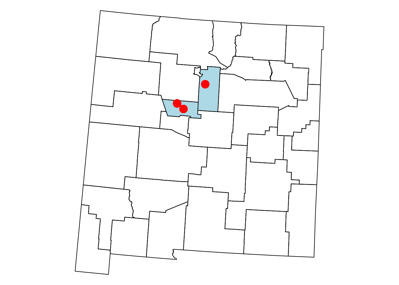
Figure 8.4: Subset of the nm layer based on intersection with airports
What will be the result of
airports[nm, ]?
What will be the result of
nm[nm[20, ], ]?
8.3 Geometric calculations
8.3.1 Introduction
Geometric operations on vector layers can conceptually be divided into three groups, according to their output:
- Numeric values (Section 8.3.2)—Functions that summarize geometrical properties of:
- Logical values (Section 8.3.3)—Functions that evaluate whether a certain condition holds true, regarding:
- A single layer—e.g., geometry is valid
- A pair of layers—e.g., feature A intersects feature B (Section 8.3.3)
- Spatial layers (Section 8.3.4)—Functions that create a new layer based on:
The following three sections elaborate and give examples of numeric (Section 8.3.2), logical (Section 8.3.3) and spatial (Section 8.3.4) geometric calculations on vector layers.
8.3.2 Numeric geometric calculations
8.3.2.1 Introduction
There are several functions to calculate numeric geometric properties of vector layers in package sf:
The first four are operation applicable for individual layers, while st_distance is applicable to pairs of layers. The next two sections give an example from each category: st_area for individual layers (Section 8.3.2.2) and st_distance for pairs of layers (Section 8.3.2.3).
8.3.2.2 Area
The st_area function returns the area of each feature or geometry. For example, we can use st_area to calculate the area of each feature in the county layer (i.e., each county):
county$area = st_area(county)
county$area[1:6]
## Units: [m^2]
## [1]  2451875694  1941109814  1077788608  1350475635 16416571545  2626706989
The result is an object of class units, which is basically a numeric vector associated with the units of measurement:
CRS units (e.g., meters) are used by default in length, area and distance calculations. For example, the units of measurement in the US National Atlas CRS are meters, which is why the area values are returned in \(m^2\) units.
We can convert units objects to different units with set_units from package units (run valid_udunits() to see the list of available units). For example, here is how we can convert the area column from \(m^2\) to \(km^2\) units:
library(units)
county$area = set_units(county$area, "km^2")
county$area[1:6]
## Units: [km^2]
## [1]  2451.876  1941.110  1077.789  1350.476 16416.572  2626.707
Dealing with units, rather than numeric values has several advantages:
- We don’t need to remember, or somehow encode, the units of measurement (e.g., name the column
area_m2) since they are already binded with the values. - We don’t need to remember the coefficients for conversion between one unit to another and avoid making mistakes in those conversions.
- We can keep track of the units when making numeric calculations. For example, if we divide a numeric value by \(km^2\), the result is going to be associated with units of density: \(km^{-2}\) (Section 8.5).
If necessary, however, we can always convert units to an ordinary numeric vector with as.numeric:
The calculated county area attribute values are visualized in Figure 8.5:
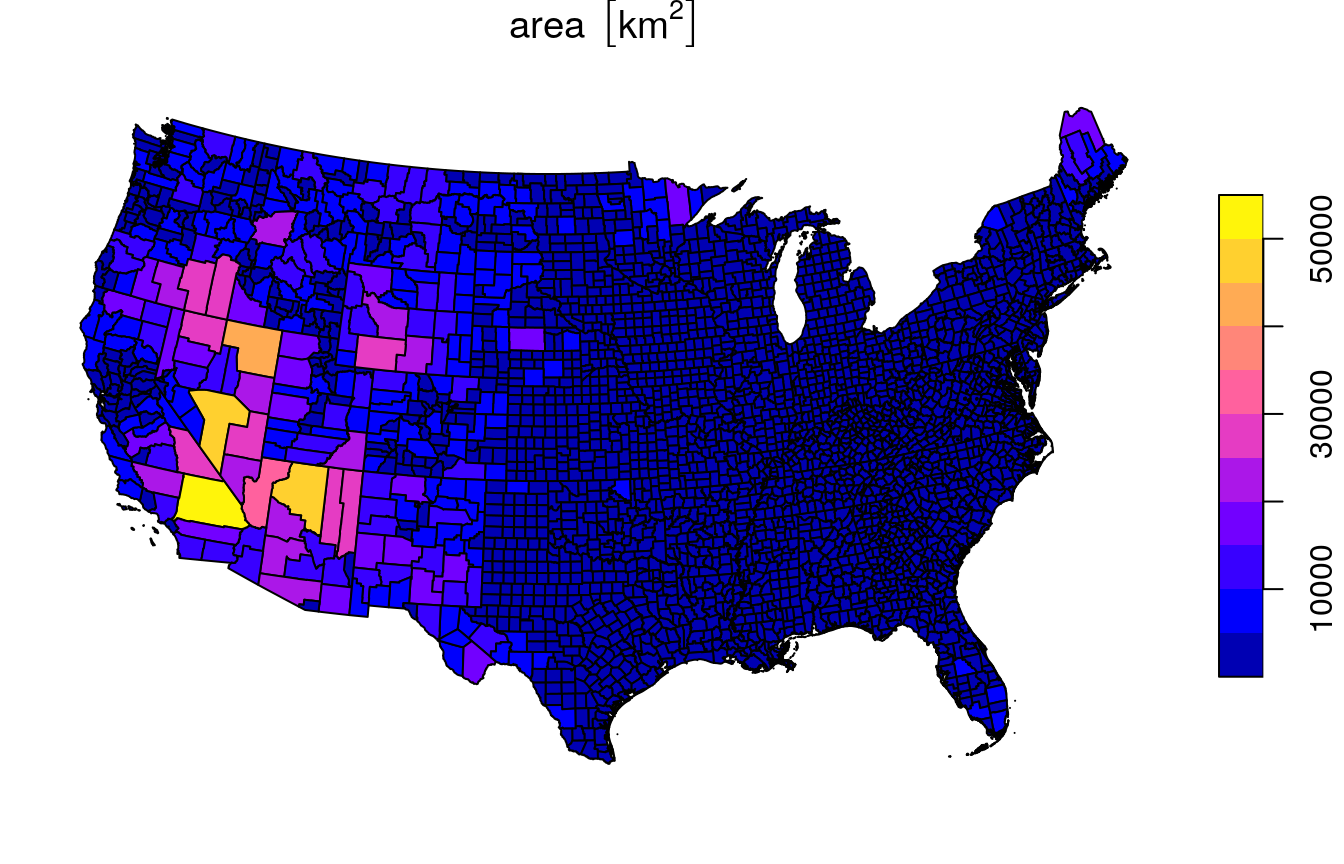
Figure 8.5: Calculated area attribute
8.3.2.3 Distance
An example of a numeric operator on a pair of geometries is geographical distance. Distances can be calculated using function st_distance. For example, the following expression calculates the distance between each feature in airports and each feature in nm:
The result is a matrix of units values:
d[, 1:6]
## Units: [m]
##          [,1]     [,2]      [,3]      [,4]      [,5]      [,6]
## [1,] 266778.9 140470.5 103328.22 140913.62 175353.34 121934.94
## [2,] 275925.0 120879.9  93753.25 141511.80 177624.40 125327.45
## [3,] 197540.4 145580.9  34956.53  62231.01  96549.17  43630.68
In the distance matrix resulting from st_distance(x, y):
- Rows refer to features of
x, e.g.,airports - Columns refer to features of
y, e.g.,nm
Therefore, the matrix dimensions are equal to c(nrow(x), nrow(y)):
Just like areas (Section 8.3.2.2), distances can be converted to different units with set_units. For example, the following expression converts the distance matrix d from \(m\) to \(km\):
d = set_units(d, "km")
d[, 1:6]
## Units: [km]
##          [,1]     [,2]      [,3]      [,4]      [,5]      [,6]
## [1,] 266.7789 140.4705 103.32822 140.91362 175.35334 121.93494
## [2,] 275.9250 120.8799  93.75325 141.51180 177.62440 125.32745
## [3,] 197.5404 145.5809  34.95653  62.23101  96.54917  43.63068
To work with the distance matrix, it can be convenient to set row and column names. We can use any of the unique attributes of x and y, such as airport names and county names:
rownames(d) = airports$name
colnames(d) = nm$NAME_2
d[, 1:6]
## Units: [km]
##                              Union San Juan Rio Arriba      Taos    Colfax
## Albuquerque International 266.7789 140.4705  103.32822 140.91362 175.35334
## Double Eagle II           275.9250 120.8799   93.75325 141.51180 177.62440
## Santa Fe Municipal        197.5404 145.5809   34.95653  62.23101  96.54917
##                                Mora
## Albuquerque International 121.93494
## Double Eagle II           125.32745
## Santa Fe Municipal         43.63068
Once row and column names are set, it is more convenient to find out the distance between a specific airport and a specific county:
8.3.3 Logical geometric calculations
Given two layers, x and y, the following logical geometric functions check whether each feature in x maintains the specified relation with each feature in y:
st_intersectsst_disjointst_touchesst_crossesst_withinst_containsst_overlapsst_coversst_covered_byst_equalsst_equals_exact
The definitions of the relations evaluated by each of those functions can be found in the Spatial Predicates entry in Wikipedia.
When specifying sparse=FALSE the functions return a logical matrix. Each element i,j in the matrix is TRUE when f(x[i], y[j]) is TRUE. For example, the following expression creates a matrix of intersection relations between counties in nm:
int = st_intersects(nm, nm, sparse = FALSE)
int[1:4, 1:4]
##       [,1]  [,2]  [,3]  [,4]
## [1,]  TRUE FALSE FALSE FALSE
## [2,] FALSE  TRUE  TRUE FALSE
## [3,] FALSE  TRUE  TRUE  TRUE
## [4,] FALSE FALSE  TRUE  TRUE
Figure 8.6 shows two matrices of spatial relations between counties in New Mexico: st_intersects (left) and st_touches (right).
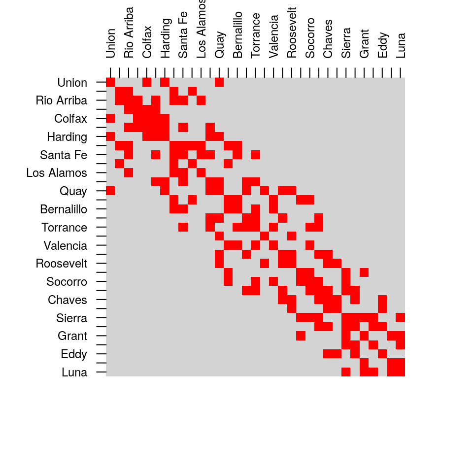
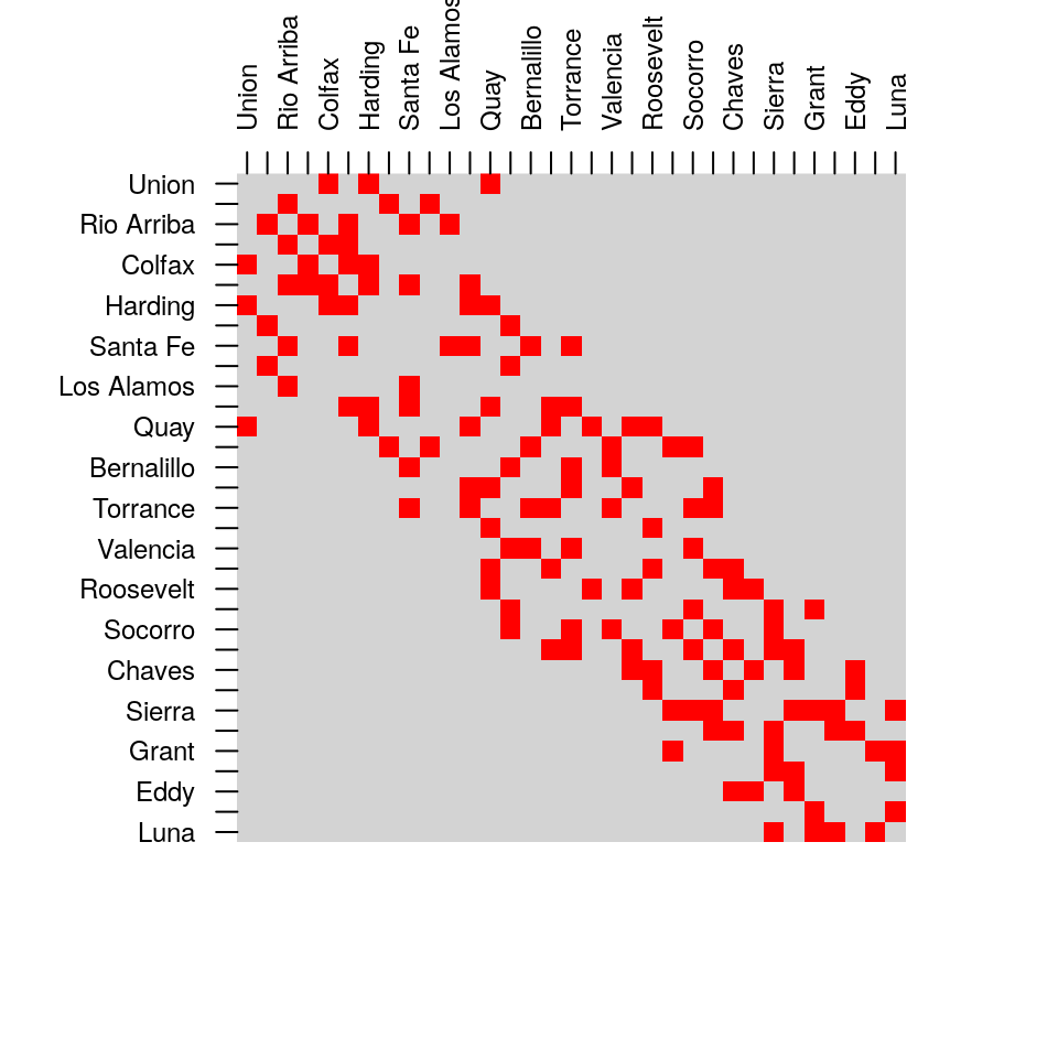
Figure 8.6: Spatial relations between counties in New Mexico, st_intersects (left) and st_touches (right)
How can we calculate
airportscount per county innm, usingst_intersects(Figure 8.7)?
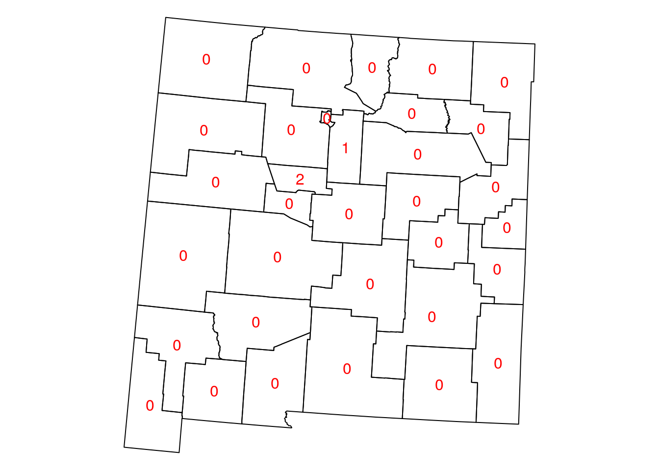
Figure 8.7: Airport count per county in New Mexico
8.3.4 Spatial geometric calculations
8.3.4.1 Introduction
The sf package provides common geometry-generating functions applicable to individual geometries, such as:
st_centroid—Section 8.3.4.2st_buffer—Section 8.3.4.5st_convex_hull—Section 8.3.4.7st_voronoist_sample
What each function does is illustrated in Figure 8.8.

Figure 8.8: Geometry-generating operations on individual layers
Additionally, the st_cast function is used to transform geometries from one type to another (Figure 7.8), which can also be considred as geometry generation (Section 8.3.4.4). The st_union and st_combine functions are used to combine multiple geometries into one, possibly dissolving their borders (Section 8.3.4.3).
Finally, the geometry-generating functions operate on pairs of geometries (Section 8.3.4.6) include:
st_intersectionst_differencest_sym_differencest_union
We elaborate on these functions in the following Sections 8.3.4.2–8.3.4.7.
8.3.4.2 Centroids
For example, the following expression uses st_centroid to create a layer of county centroids:
The nm layer along with the calculated centroids is shown in Figure 8.9:
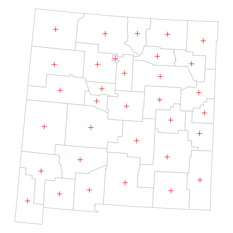
Figure 8.9: Centroids of New Mexico counties
8.3.4.3 Combining and dissolving
The st_combine and st_union functions can be used to combine multiple geometries into a single one. The difference is that st_combine only combines the geometries, while st_union also dissolves internal borders.
To understand what each function does, let’s examine the result of applying them on nm:
st_combine(nm)
## Geometry set for 1 feature
## geometry type:  MULTIPOLYGON
## dimension:      XY
## bbox:           xmin: -863763.9 ymin: -1478601 xmax: -267074.1 ymax: -845634.3
## projected CRS:  US National Atlas Equal Area
## MULTIPOLYGON (((-267074.1 -884175.1, -267309.2 ...st_union(nm)
## Geometry set for 1 feature
## geometry type: POLYGON
## dimension: XY
## bbox: xmin: -863763.9 ymin: -1478601 xmax: -267074.1 ymax: -845634.3
## projected CRS: US National Atlas Equal Area
## POLYGON ((-852411.9 -1350402, -850603.1 -133127...The results are plotted in Figure 8.10:
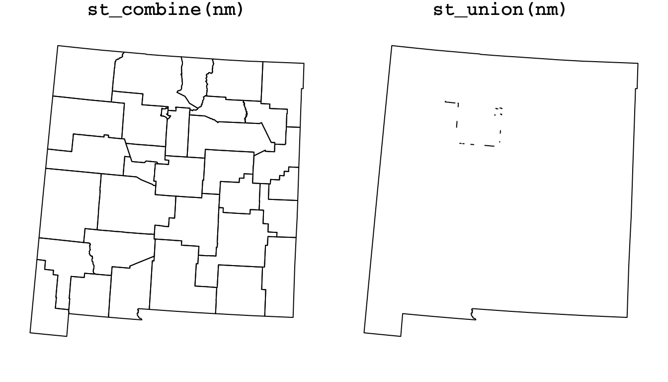
Figure 8.10: Combining (st_combine) and dissolving (st_union) polygons
What is the class of the resulting objects? Why? What happened to the original
nmattributes?
Why did
st_combinereturn aMULTIPOLYGON, whilest_unionreturnedPOLYGON?
Why do you think there are internal “patches” in the result of
st_union(nm)(Figure 8.10)?
Let’s solve a geometric question to practice some of the functions we learned so far. What is the distance between the centroids of California and New Jersey, in kilometers? Using [, st_union, st_centroid and st_distance, we can calculate it as follows:
# Subsetting
ca = county[county$NAME_1 == "California", ]
nj = county[county$NAME_1 == "New Jersey", ]

# Calculating centroids
ca_ctr = st_centroid(st_union(ca))
nj_ctr = st_centroid(st_union(nj))

# Calculating distance
d = st_distance(ca_ctr, nj_ctr)

# Converting to kilometers
set_units(d, "km")
## Units: [km]
##         [,1]
## [1,] 3846.64
Note that we are using st_union to combine the county polygons into a single geometry, so that we can calculate the centroid of the state polygon, as a whole.
We can use the c function to combine two geometry columns into one (long) geometry column, which is very similar to the way c works on vectors:
p = c(ca_ctr, nj_ctr)
p
## Geometry set for 2 features
## geometry type:  POINT
## dimension:      XY
## bbox:           xmin: -1707694 ymin: -667480.7 xmax: 2111204 ymax: -206332.8
## projected CRS:  US National Atlas Equal Area
## POINT (-1707694 -667480.7)
## POINT (2111204 -206332.8)
The centroids we calculated can be displayed as follows (Figure 8.11):
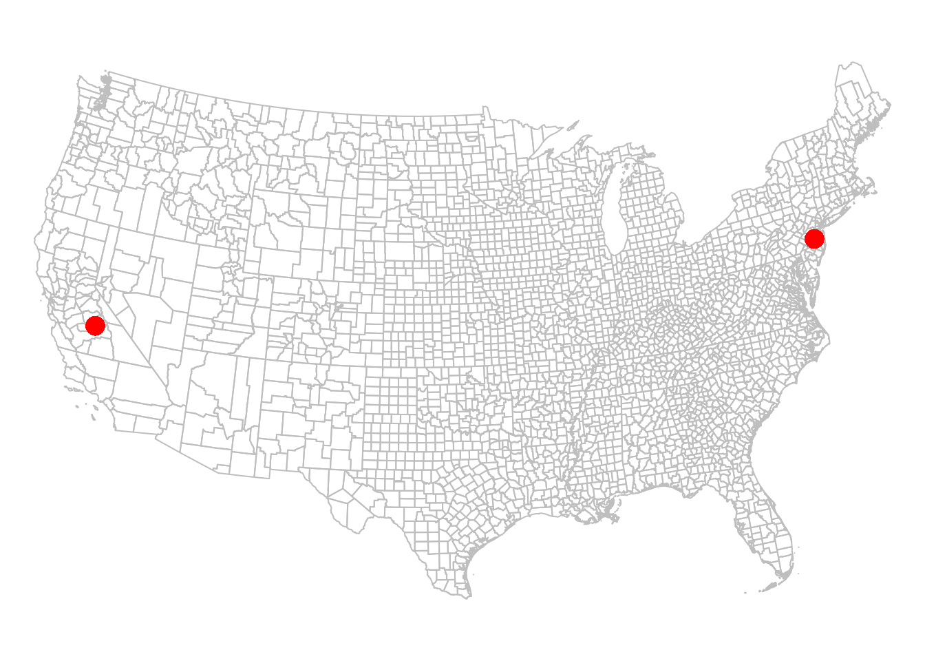
Figure 8.11: California and New Jersey centroids
How can we draw a line line between the centroids, corresponding to the distance we just calculated (Figure 8.12)?
First, we can use st_combine to transform the points into a single MULTIPOINT geometry. Remember, the st_combine function is similar to st_union, but only combines and does not dissolve.
p = st_combine(p)
p
## Geometry set for 1 feature
## geometry type:  MULTIPOINT
## dimension:      XY
## bbox:           xmin: -1707694 ymin: -667480.7 xmax: 2111204 ymax: -206332.8
## projected CRS:  US National Atlas Equal Area
## MULTIPOINT ((-1707694 -667480.7), (2111204 -206...
Do you think the results of
st_union(p)andst_combine(p)will be different, and if so in what way?
What is left to be done is to transform the MULTIPOINT geometry to a LINESTRING geometry, which is what we learn next (Section 8.3.4.4).
8.3.4.4 Geometry casting
The st_cast function can be used to convert between different geometry types. The st_cast function accepts:
- The input layer
- The destination geometry type
For example, we can use st_cast to convert our MULTIPOINT geometry p to a LINESTRING geometry l:
l = st_cast(p, "LINESTRING")
l
## Geometry set for 1 feature
## geometry type:  LINESTRING
## dimension:      XY
## bbox:           xmin: -1707694 ymin: -667480.7 xmax: 2111204 ymax: -206332.8
## projected CRS:  US National Atlas Equal Area
## LINESTRING (-1707694 -667480.7, 2111204 -206332.8)
Each MULTIPOINT geometry is replaced with a LINESTRING geometry, comprising a line that goes through all points from first to last. In this case, p contains just one MULTIPOINT geometry that contains two points. Therefore, the resulting geometry column l contains one LINESTRING geometry with a straight line.
The line we calculated is shown in Figure 8.12:
plot(st_geometry(county), border = "grey")
plot(st_geometry(ca_ctr), col = "red", pch = 16, cex = 2, add = TRUE)
plot(st_geometry(nj_ctr), col = "red", pch = 16, cex = 2, add = TRUE)
plot(l, col = "red", add = TRUE)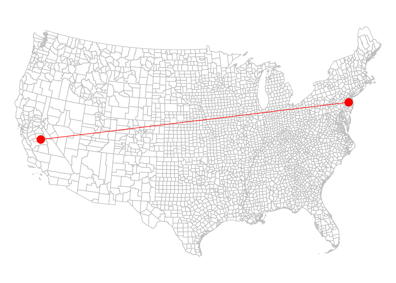
Figure 8.12: California and New Jersey centroids, with a line
It is important to note that note every conversion operation is possible. Meaningless st_cast operations will fail with an error message. For example, a LINESTRING composed of just two points cannot be converted to a POLYGON:
8.3.4.5 Buffers
Another example of a function that generates now geometries based on individual input geometries is st_buffer, which calculates buffers.
For example, here is how we can calculate 100 \(km\) buffers around the airports. Note that the st_buffer requires buffer distance (dist), which can be passed as numeric (in which case CRS units are assumed) or as units:
The buffered layer is shown in Figure 8.13:
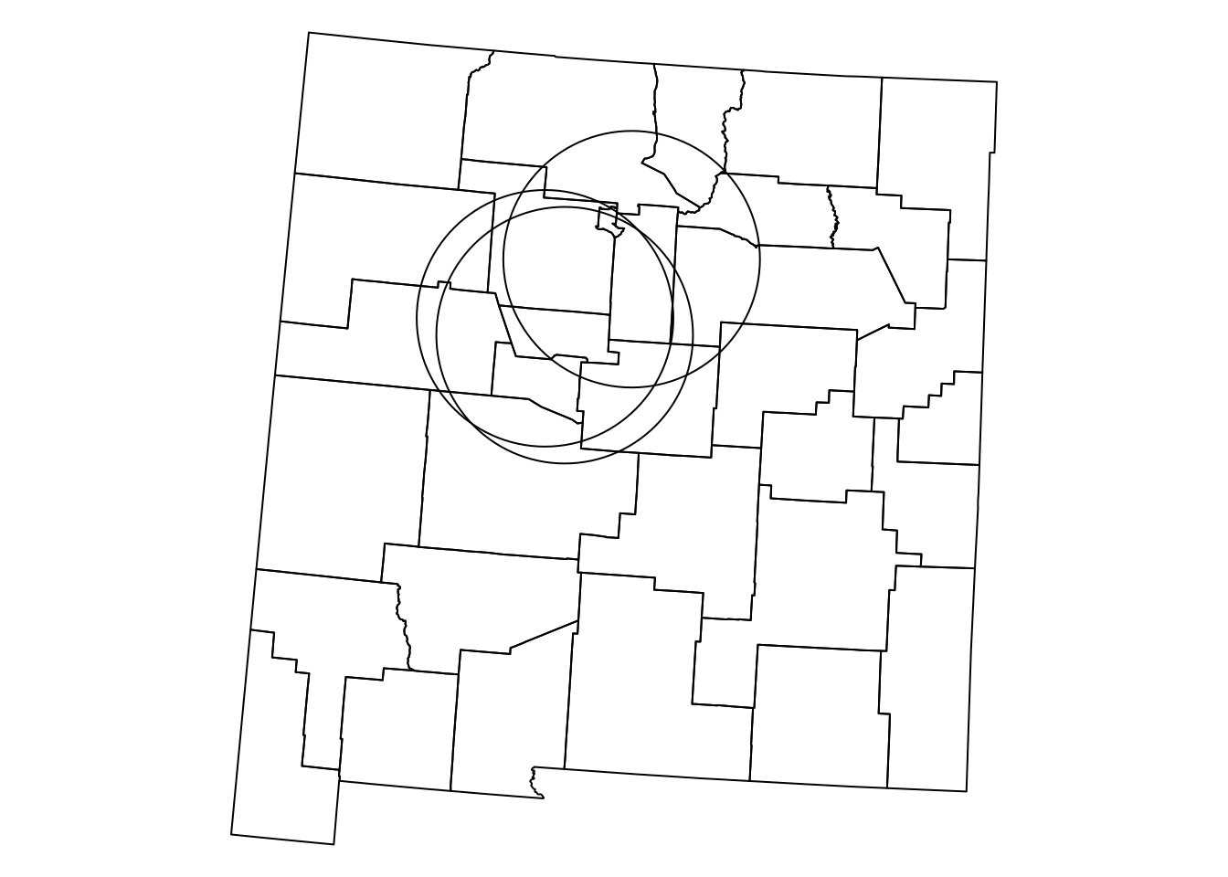
Figure 8.13: airports buffered by 100 km
8.3.4.6 Geometry generation from pairs
There are four geometry-generating functions that work on pairs of input geometries:
st_intersectionst_differencest_sym_differencest_union
Figure 8.14 shows what each of the four functions does.
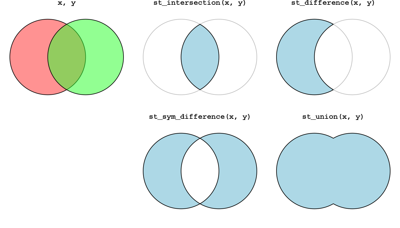
Figure 8.14: Geometry-generating operations on pairs of layers
For example, suppose that we need to calculate the area that is within 100 \(km\) range of all three airports at the same time? We can find the area of intersection of the three airports, using st_intersection:
inter1 = st_intersection(airports_100[1, ], airports_100[2, ])
inter2 = st_intersection(inter1, airports_100[3, ])The result is shown in Figure 8.15:
plot(st_geometry(nm))
plot(st_geometry(airports_100), add = TRUE)
plot(inter2, col = "lightblue", add = TRUE)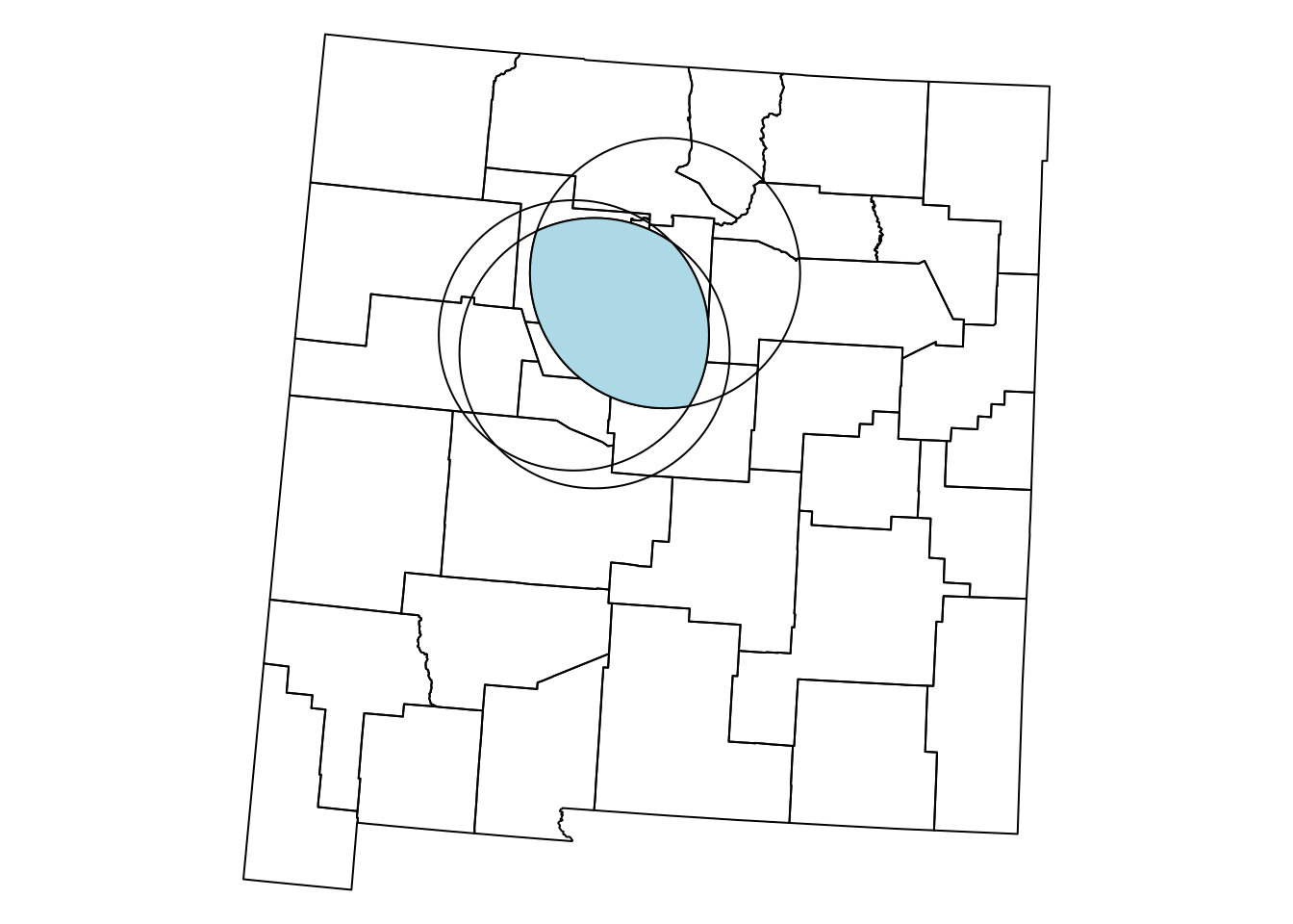
Figure 8.15: The intersection of three airports buffers
How can we calculate the area that is at within 100 \(km\) range of at least one of the three airports? As shown in Section 8.3.4.3, st_union can be applied on an individual layer, in which case it returns the (dissolved) union of all geometries:
The result is shown in Figure 8.16:
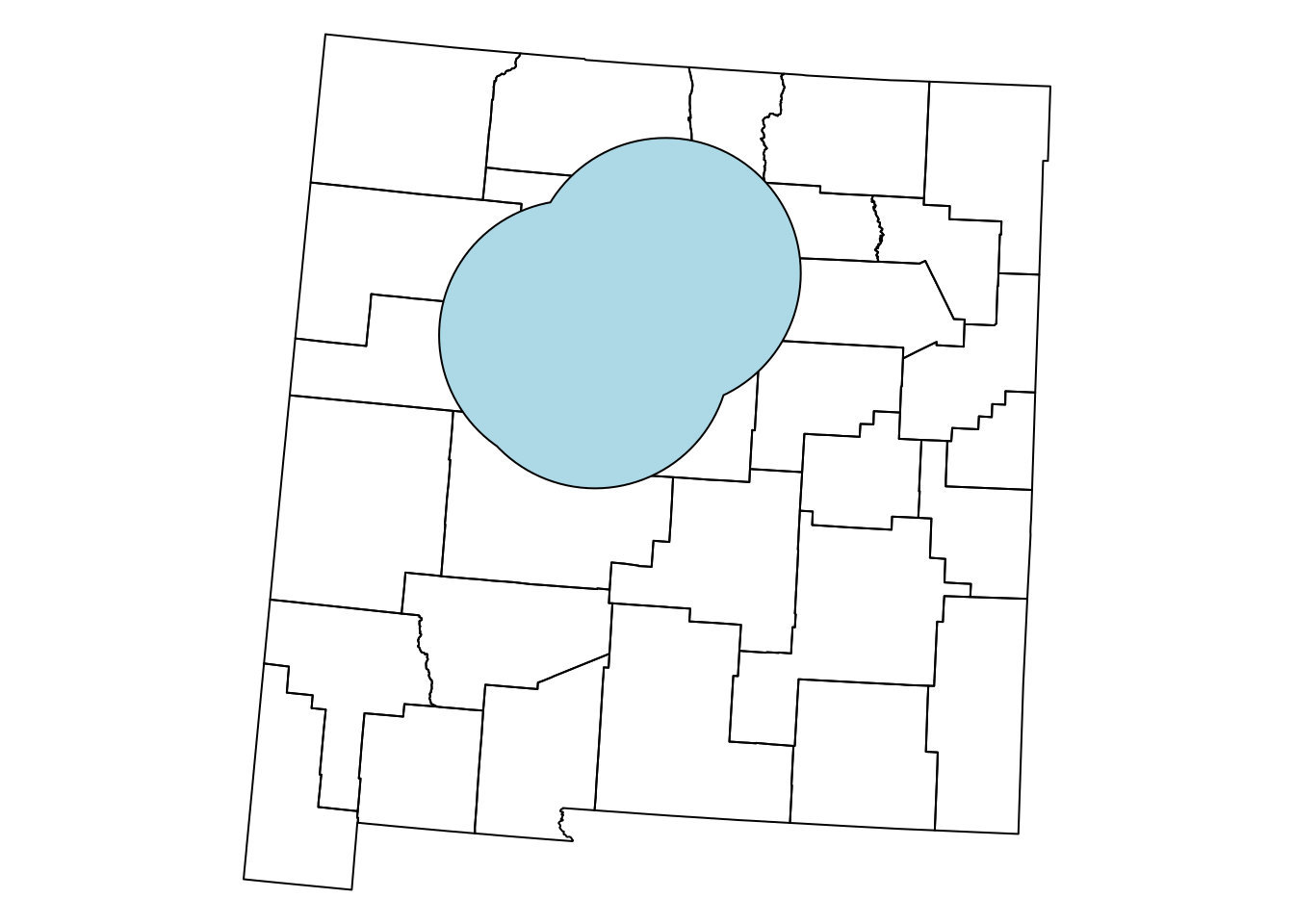
Figure 8.16: The union of three airports buffers
8.3.4.7 Convex hull
The Convex Hull of a set \(X\) of points is the smallest convex set that contains \(X\). The convex hull may be visualized as the shape resulting when stretching a rubber band around \(X\), then releasing it until it shrinks to minimal size (Figure 8.17).
![Convex Hull: elastic-band analogy^[https://en.wikipedia.org/wiki/Convex_hull]](images/lesson_08_convex_hull.png)
Figure 8.17: Convex Hull: elastic-band analogy40
For example, the following expression calculates the convex hull (per feature) in nm1:
The resulting layer is shown in red in Figure 8.18:
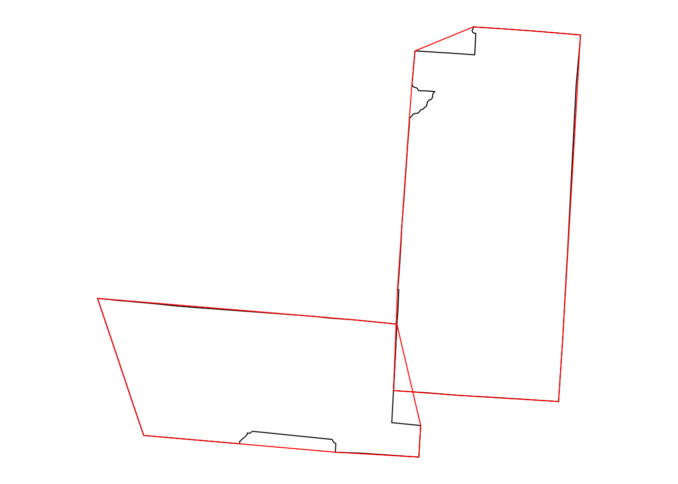
Figure 8.18: Convex hull polygons for two counties in New Mexico
How can we calculate the convex hull of all polygons in
nm1(Figure 8.19)?

Figure 8.19: Convex Hull of multiple polygons
Here is another question to practice the geometric operations we learned in this chapter. Suppose we build a tunnel, 10 \(km\) wide, between the centroids of "Harding" and "Sierra" counties in New Mexico. Which counties does the tunnel go through? The following code gives the result. Take a moment to go over it and make sure you understand what happens in each step:
w = nm[nm$NAME_2 %in% c("Harding", "Sierra"), ]
w_ctr = st_centroid(w)
w_ctr_buf = st_buffer(w_ctr, dist = 5000)
w_ctr_buf_u = st_combine(w_ctr_buf)
w_ctr_buf_u_ch = st_convex_hull(w_ctr_buf_u)
nm_w = nm[w_ctr_buf_u_ch, ]
nm_w$NAME_2
## [1] "Harding"    "San Miguel" "Guadalupe"  "Torrance"   "Socorro"
## [6] "Lincoln"    "Sierra"
Figure 8.20 shows the calculated tunnel geometry and highlights the counties that the tunnel goes through. We also use the text function to draw text labels. The function accepts the matrix of coordinates where labels should be drawn (e.g., county centroid coordinates) and the corresponding character vector of lables (e.g., county names):
plot(st_geometry(nm_w), border = NA, col = "lightblue")
plot(st_geometry(nm), add = TRUE)
plot(st_geometry(w_ctr_buf_u_ch), add = TRUE)
text(st_coordinates(st_centroid(nm_w)), nm_w$NAME_2)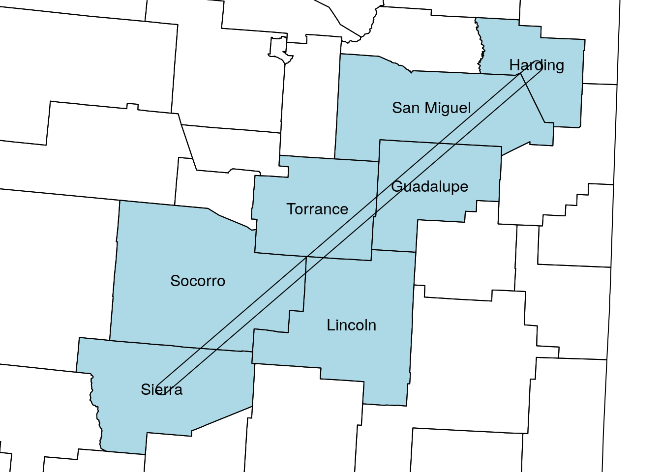
Figure 8.20: Tunnel between “Sierra” and “Harding” county centroids
How is the area of the “tunnel” divided between the various counties that it crosses? We can use the st_intersection(x, y) to calculate all intersections between the tunnel polygon and the county polygons:
int = st_intersection(w_ctr_buf_u_ch, nm_w)
int
## Geometry set for 7 features
## geometry type:  POLYGON
## dimension:      XY
## bbox:           xmin: -677075.1 ymin: -1293982 xmax: -340138.8 ymax: -1002634
## projected CRS:  US National Atlas Equal Area
## First 5 geometries:
## POLYGON ((-359510.4 -1013406, -348484.4 -100391...
## POLYGON ((-430575.6 -1074562, -359510.4 -101340...
## POLYGON ((-484643 -1121091, -430575.6 -1074562,...
## POLYGON ((-545452.3 -1173421, -484643 -1121091,...
## POLYGON ((-638440.3 -1253443, -546193.4 -117405...
Then, we can divide the area of each tunnel part by the total area of the tunnel to get the proportions:
area = st_area(int)
area
## Units: [m^2]
## [1]  199064581  872145769  813577715  702562404 1119738156  108077571  575538789
prop = area / sum(area)
prop
## Units: [1]
## [1] 0.04533773 0.19863456 0.18529546 0.16001130 0.25502469 0.02461508 0.13108118
The proportions can be displayed as text labels using the text function (Figure 8.21):
plot(st_geometry(nm_w), border = "darkgrey")
plot(int, col = hcl.colors(7, "Set3"), border = "grey", add = TRUE)
text(st_coordinates(st_centroid(int)), paste0(round(prop, 2)*100, "%"), cex = 1.5)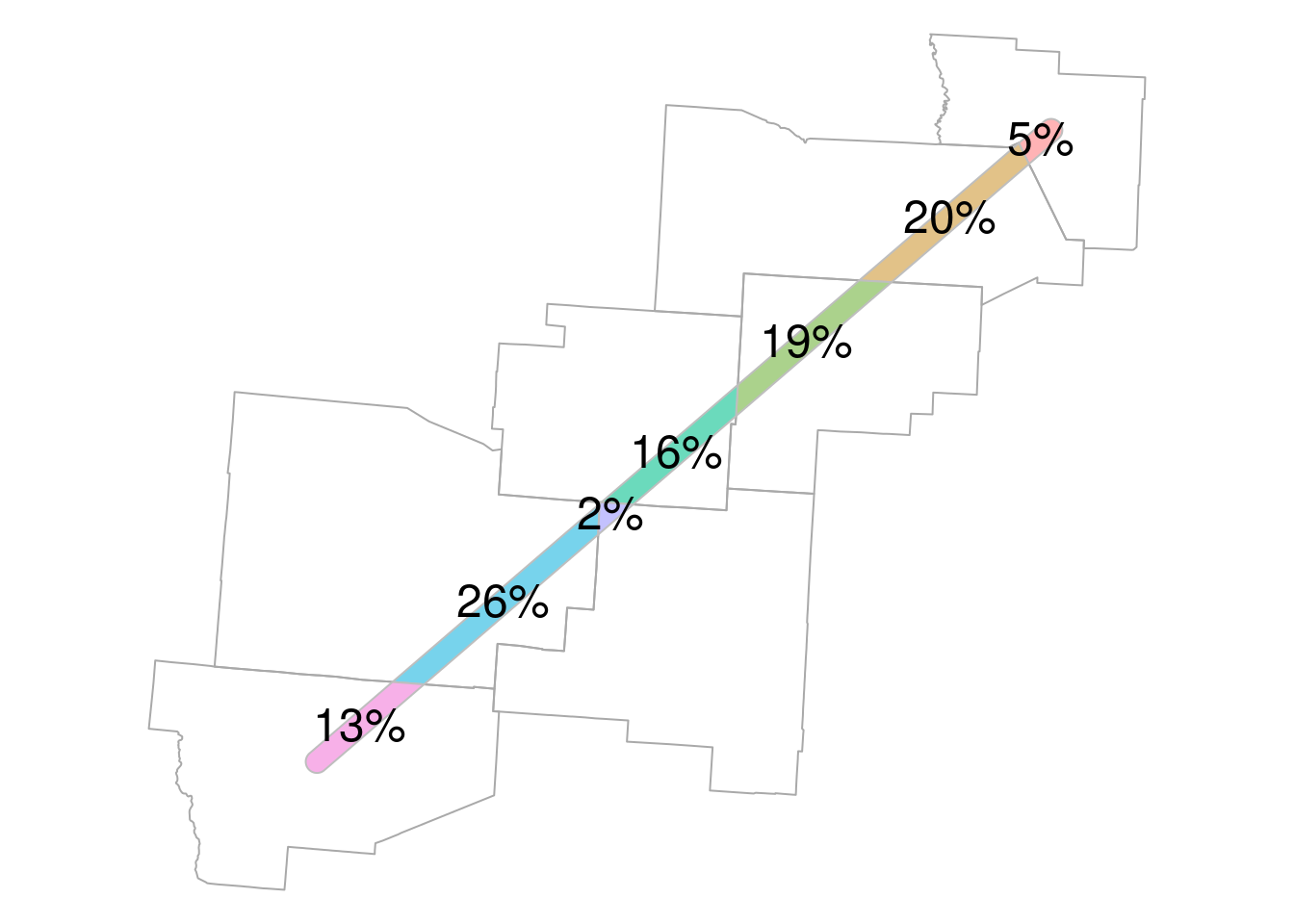
Figure 8.21: Proportion of tunnel area within each county
8.4 Vector layer aggregation
We don’t always have to dissolve all features—we can also dissolve by attribute or by location. To demonstrate dissolving by attribute, also known as aggregation, let’s take a subset with all counties of Arizona and Utah:
The selected counties are shown in Figure 8.22:
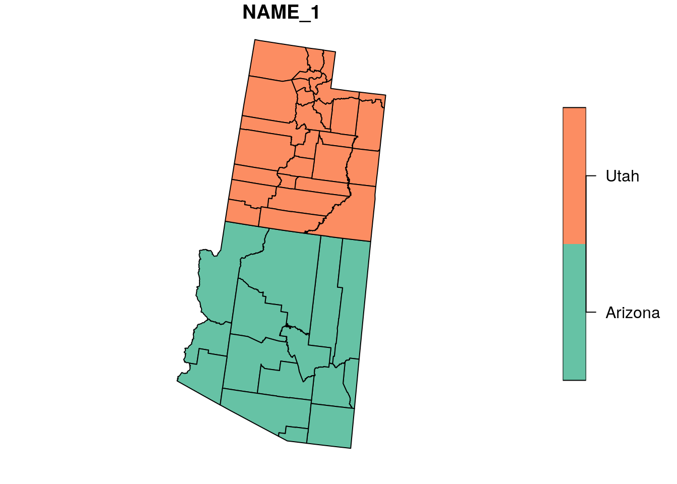
Figure 8.22: Subset of two states from county
As shown previously (Section 8.3.4.3), we can dissolve all features into a single geometry with st_union:
s1 = st_union(s)
s1
## Geometry set for 1 feature
## geometry type:  POLYGON
## dimension:      XY
## bbox:           xmin: -1389076 ymin: -1470784 xmax: -757960.3 ymax: -235145.7
## projected CRS:  US National Atlas Equal Area
## POLYGON ((-852411.9 -1350402, -852611 -1352512,...
The dissolved geometry is shown in Figure 8.23:
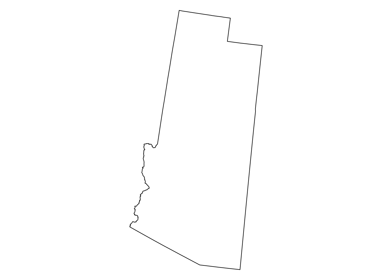
Figure 8.23: Union of all counties in s
Aggregating/dissolving by attributes can be done with aggregate41, which accepts the following arguments:
x—Thesflayer being dissolvedby—A correspondingdata.framedetermining the groupsFUN—The function to be applied on each attribute inx
For example, the following expression dissolves the layer s, summing the area attribute by state:
s2 = aggregate(x = s[, "area"], by = st_drop_geometry(s[, "NAME_1"]), FUN = sum)
s2
## Simple feature collection with 2 features and 2 fields
## Attribute-geometry relationship: 0 constant, 1 aggregate, 1 identity
## geometry type:  POLYGON
## dimension:      XY
## bbox:           xmin: -1389076 ymin: -1470784 xmax: -757960.3 ymax: -235145.7
## projected CRS:  US National Atlas Equal Area
##    NAME_1            area                       geometry
## 1 Arizona 295423.1 [km^2] POLYGON ((-852411.9 -135040...
## 2    Utah 219634.4 [km^2] POLYGON ((-1011317 -819521....
The unit of measurement is lost, so we need to reconstruct it:
s2$area = set_units(as.numeric(s2$area), "km^2")
s2
## Simple feature collection with 2 features and 2 fields
## Attribute-geometry relationship: 0 constant, 0 aggregate, 1 identity, 1 NA's
## geometry type:  POLYGON
## dimension:      XY
## bbox:           xmin: -1389076 ymin: -1470784 xmax: -757960.3 ymax: -235145.7
## projected CRS:  US National Atlas Equal Area
##    NAME_1            area                       geometry
## 1 Arizona 295423.1 [km^2] POLYGON ((-852411.9 -135040...
## 2    Utah 219634.4 [km^2] POLYGON ((-1011317 -819521....
The result is shown in Figure 8.24:
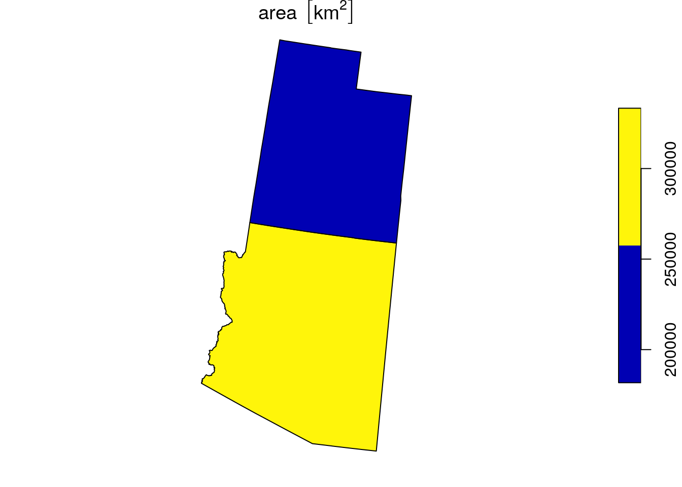
Figure 8.24: Union by state name of s
8.5 Join by attributes
We can join a vector layer and a table exactly the same way as two tables, e.g., using the merge function (Section 4.6). This is analogous to the “Join attributes from a table” workflow in ArcGIS (Figure 8.25).
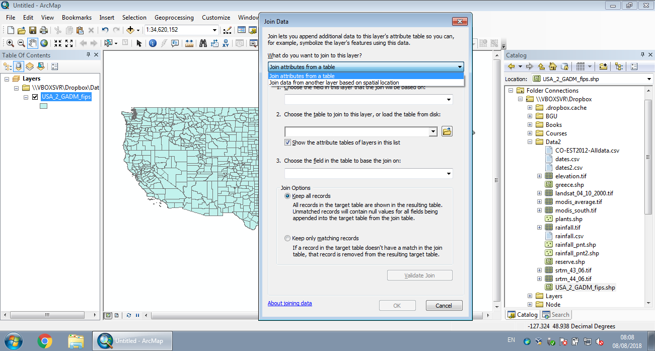
Figure 8.25: Join by attributes in ArcGIS
In the next example we will join county-level demographic data, from CO-EST2012-Alldata.csv, with the county layer. The join will be based on the common Federal Information Processing Standards (FIPS) code of each county.
First, let’s read the CO-EST2012-Alldata.csv file into a data.frame named dat:
And subset the columns we are interested in:
STATE—State codeCOUNTY—County codeCENSUS2010POP—Population size in 2010
dat = dat[, c("STATE", "COUNTY", "CENSUS2010POP")]
head(dat)
##   STATE COUNTY CENSUS2010POP
## 1     1      0       4779736
## 2     1      1         54571
## 3     1      3        182265
## 4     1      5         27457
## 5     1      7         22915
## 6     1      9         57322
Records where COUNTY code is 0 are state sums. We need to remove the state sums and keep just the county-level records:
dat = dat[dat$COUNTY != 0, ]
head(dat)
##   STATE COUNTY CENSUS2010POP
## 2     1      1         54571
## 3     1      3        182265
## 4     1      5         27457
## 5     1      7         22915
## 6     1      9         57322
## 7     1     11         10914
The FIPS code is a character value with five digits, where the first two digits are the state code and the last three digits are the county code:
To get the corresponding county FIPS codes in dat, we need to:
- Standardize the state code to a two-digit code
- Standardize the county code to three-digit code
- Paste the two into a five-digit FIPS code
The formatC function can be used to format numeric values into different formats, using different “scenarios”. The “add leading zeros” scenario is specified using width=n, where n is the required number of digits, and flag="0":
dat$STATE = formatC(dat$STATE, width = 2, flag = "0")
dat$COUNTY = formatC(dat$COUNTY, width = 3, flag = "0")
dat$FIPS = paste0(dat$STATE, dat$COUNTY)
Now we have a column named FIPS with exactly the same format as in the county layer:
head(dat)
##   STATE COUNTY CENSUS2010POP  FIPS
## 2    01    001         54571 01001
## 3    01    003        182265 01003
## 4    01    005         27457 01005
## 5    01    007         22915 01007
## 6    01    009         57322 01009
## 7    01    011         10914 01011
This means we can join the county layer with the dat table, based on the common column named FIPS:
county = merge(county, dat[, c("FIPS", "CENSUS2010POP")], by = "FIPS", all.x = TRUE)
county
## Simple feature collection with 3103 features and 6 fields
## geometry type:  MULTIPOLYGON
## dimension:      XY
## bbox:           xmin: -2031903 ymin: -2116922 xmax: 2516534 ymax: 732304.6
## projected CRS:  US National Atlas Equal Area
## First 10 features:
##     FIPS  NAME_1   NAME_2 TYPE_2            area CENSUS2010POP
## 1  01001 Alabama  Autauga County 1562.805 [km^2]         54571
## 2  01003 Alabama  Baldwin County 4247.589 [km^2]        182265
## 3  01005 Alabama  Barbour County 2330.135 [km^2]         27457
## 4  01007 Alabama     Bibb County 1621.356 [km^2]         22915
## 5  01009 Alabama   Blount County 1692.125 [km^2]         57322
## 6  01011 Alabama  Bullock County 1623.924 [km^2]         10914
## 7  01013 Alabama   Butler County 2013.066 [km^2]         20947
## 8  01015 Alabama  Calhoun County 1591.091 [km^2]        118572
## 9  01017 Alabama Chambers County 1557.054 [km^2]         34215
## 10 01019 Alabama Cherokee County 1549.770 [km^2]         25989
##                          geometry
## 1  MULTIPOLYGON (((1225972 -12...
## 2  MULTIPOLYGON (((1200268 -15...
## 3  MULTIPOLYGON (((1408158 -13...
## 4  MULTIPOLYGON (((1207082 -12...
## 5  MULTIPOLYGON (((1260171 -11...
## 6  MULTIPOLYGON (((1370531 -12...
## 7  MULTIPOLYGON (((1280245 -13...
## 8  MULTIPOLYGON (((1313695 -11...
## 9  MULTIPOLYGON (((1374433 -12...
## 10 MULTIPOLYGON (((1333380 -10...
Note that we are using a left join, therefore the county layer remains as is; features that do not have a matching FIPS value in dat will have NA in the new CENSUS2010POP column.
A map of the new CENSUS2010POP attribute, using the default equal breaks, is shown in Figure 8.26:
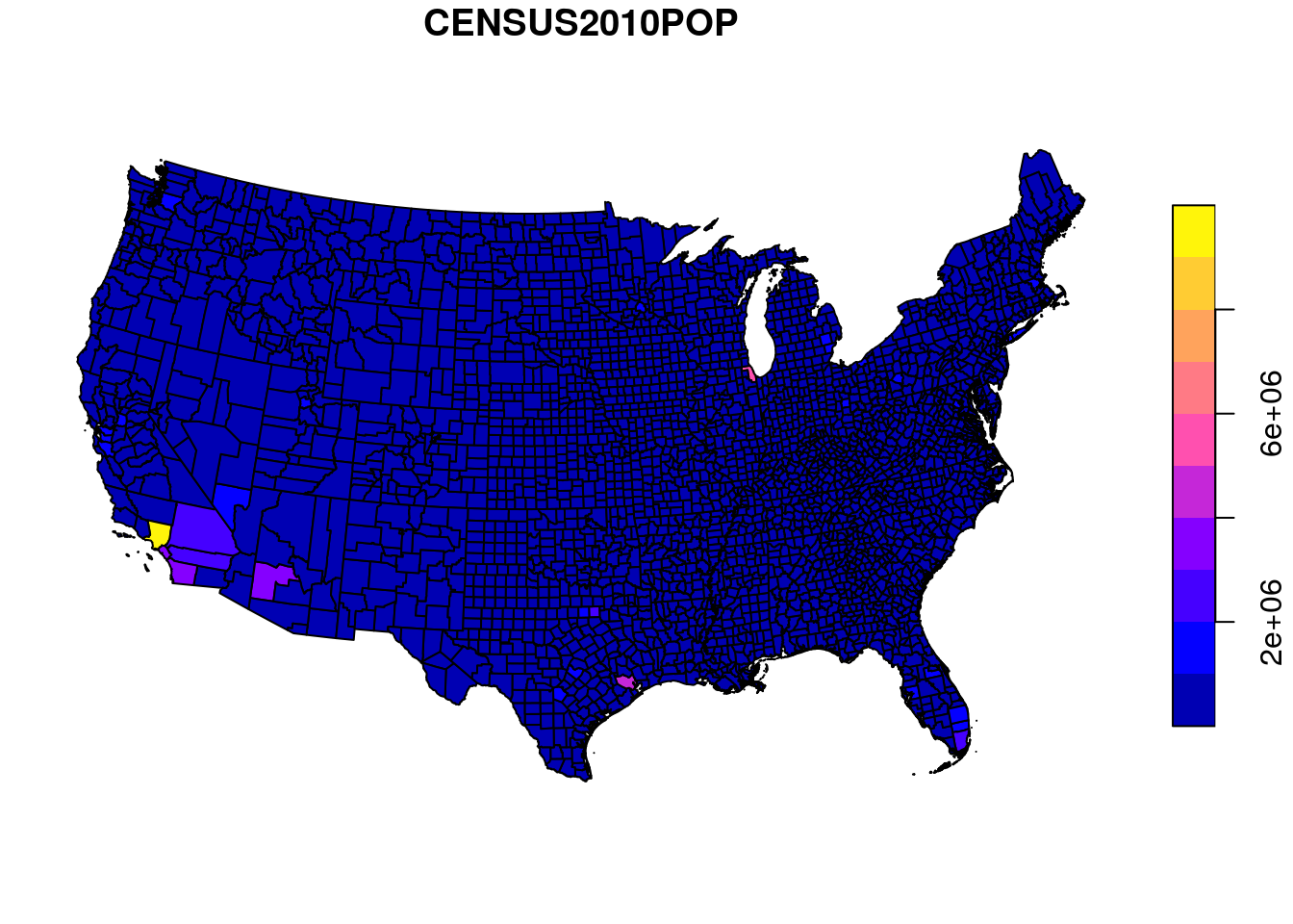
Figure 8.26: Population size per county in the US (equal breaks)
Almost all counties fall into the first category, therefore the map is uniformely colored and not very informative. A map using quantile breaks (Figure 8.27) reveals the spatial pattern of population sizes more clearly.
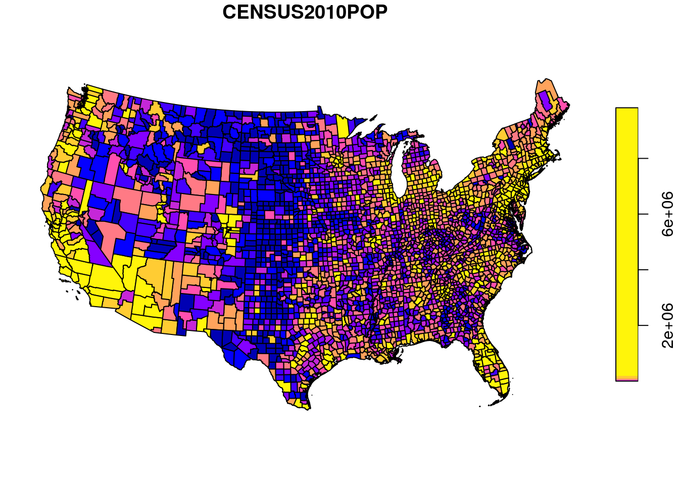
Figure 8.27: Population size per county in the US (quantile breaks)
Another issue with the map is that county population size also depends on county area, which can make the pattern misleading in case when county area sizes are variable (which they are). To safely compare the counties we need to standardize population size by county area. In other words, we need to calculate population density:
Note how the measurement units (\(km^{-2}\), i.e., count per \(km^2\)) for the new column are automatically determined based on the inputs:
The map of population densities per county is shown in Figure 8.28:
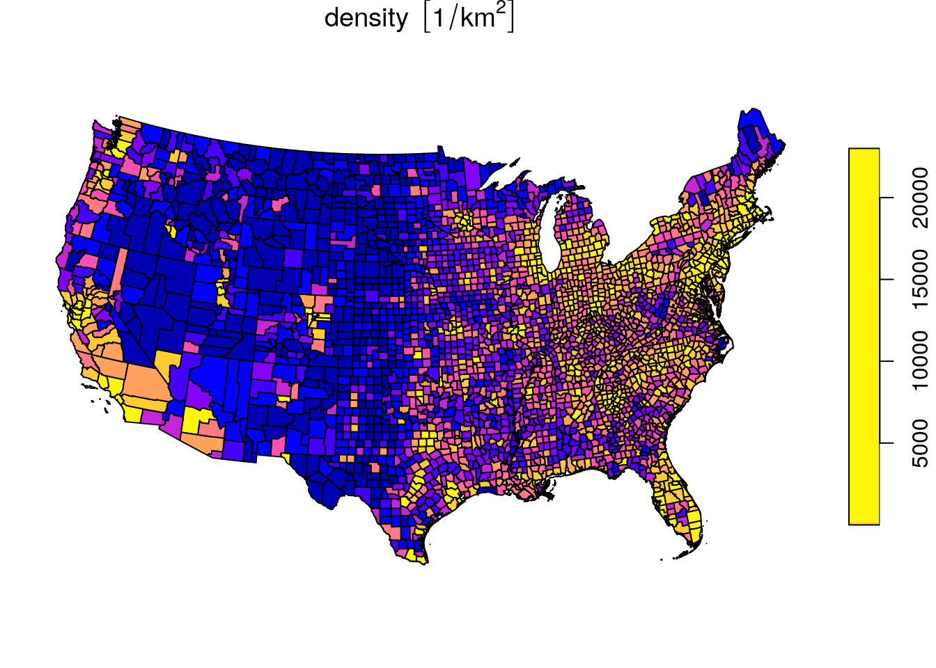
Figure 8.28: Population density in the US, quantile breaks
How many features in
countydid not have a matching FIPS code indat? What are their names?
How many features in
datdo not have a matching FIPS code incounty?
We can also calculate the average population density in the US, by dividing the total population by the total area:
This is close to the population density in 2010 according to Wikipedia, which is 40.015.
Simply averaging the density column gives an overestimation, because all counties get equal weight while in reality the smaller counties are more dense:
8.6 Recap: main data structures
Table 8.1 summarizes the main data structures we learn in this book.
| Category | Class | Chapter |
|---|---|---|
| Vector | numeric, character, logical |
2 |
| Date | Date |
3 |
| Table | data.frame |
4 |
| Matrix | matrix |
5 |
| Array | array |
5 |
| Raster | stars |
5 |
| Vector layer | sfg, sfc, sf |
7 |
| Units | units |
8 |
| List | list |
11 |
| Geostatistical model | gstat |
12 |
| Variogram model | variogramModel |
12 |
Alternatively, the
group_byandsummarizefunctions from packagedplyrcan also be used for aggregation:s2 = s %>% group_by(NAME_1) %>% summarize(area = sum(area)).↩