Chapter 10 Combining rasters and vector layers
Last updated: 2025-02-06 09:31:29
Aims
Our aims in this chapter are to learn how to:
- Crop and mask a raster according to a vector layer
- Switch from vector to raster representation, and vice versa
- Calculate a raster of distances to nearest point
- Extract raster values from locations defined by a vector layer
We will use the following R packages:
sfstarsunits
10.1 Masking and cropping rasters
10.1.1 Introduction
Masking a raster means turning pixels values outside of an area of interest—defined using a polygonal layer—into NA (Figure 10.1). Cropping a raster means deleting whole rows and/or columns, so that raster extent is reduced to a new (smaller) rectangular shape, also according to the extent of a vector layer. The [ operator can be used for masking, or for masking and cropping (the latter is the default).

Figure 10.1: Masking a raster (http://rpubs.com/etiennebr/visualraster)
10.1.2 Masking and cropping
For an example of masking and cropping, we will prepare a raster of average NDVI over the period 2000-2019, based on MOD13A3_2000_2019.tif. The following code section combines what we learned in Sections 6.3.2, 6.6.1.3 and 9.3:
library(stars)
r = read_stars('data/MOD13A3_2000_2019.tif')
names(r) = 'NDVI'
dates = read.csv('data/MOD13A3_2000_2019_dates2.csv')
dates$date = as.Date(dates$date)
r = st_set_dimensions(r, 'band', values = dates$date, names = 'time')
r = st_warp(r, crs = 32636)
r_avg = st_apply(r, c('x','y'), mean, na.rm = TRUE)
names(r_avg) = 'NDVI'
We will also read a Shapefile with a polygon of Israel borders, named israel_borders.shp:
Figure 10.2 shows the average NDVI raster and the borders polygon:
plot(r_avg, breaks = 'equal', col = function(n) hcl.colors(n, 'Spectral'), reset = FALSE)
plot(st_geometry(borders), add = TRUE)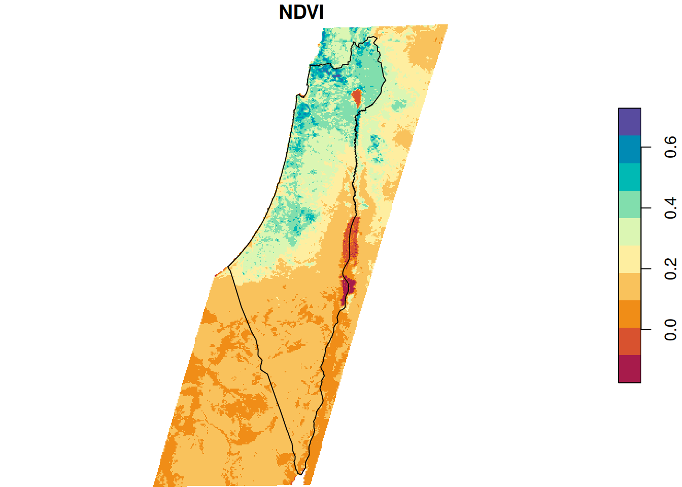
Figure 10.2: Raster and crop/mask geometry
Masking and cropping a raster, based on an sf layer, can be done with the [ operator, as follows:
As we can see in Figure 10.3, all pixels that were outside of the polygon are now NA (this is called masking). It’s difficult to see, but the raster extent is also slightly reduced according to the extent of borders (this is called cropping):
plot(r_avg, breaks = 'equal', col = function(n) hcl.colors(n, 'Spectral'), reset = FALSE)
plot(st_geometry(borders), add = TRUE)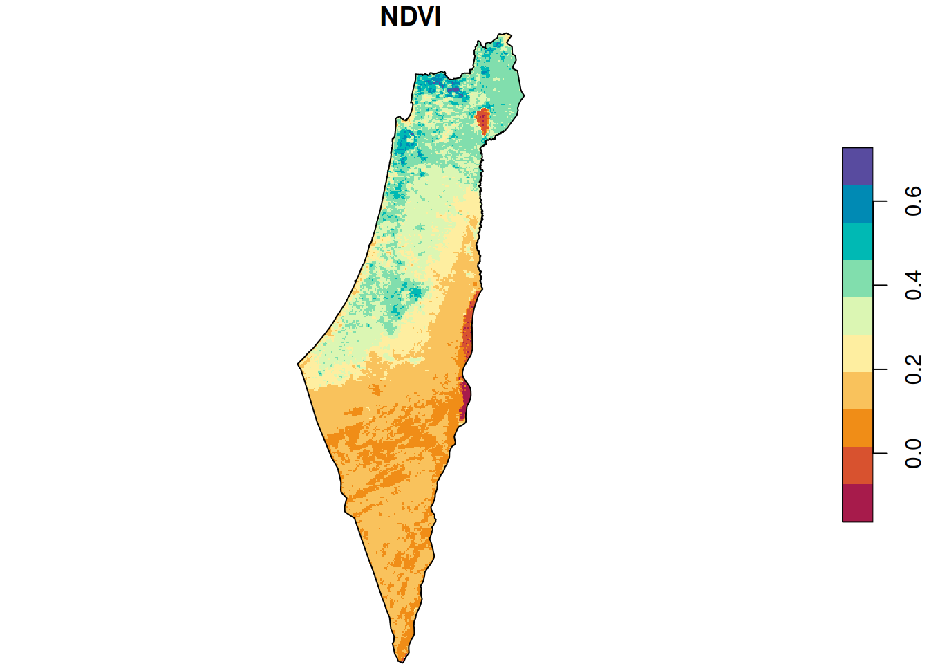
Figure 10.3: Raster after cropping and masking
Zooming in on a small portion of the masked raster demonstrates the masking algorithm. Pixels whose centroid does not intersect with the polygon are converted to NA (Figure 10.4).
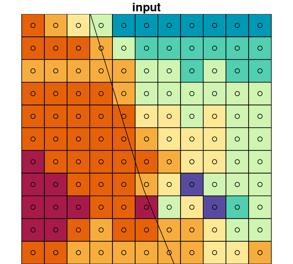
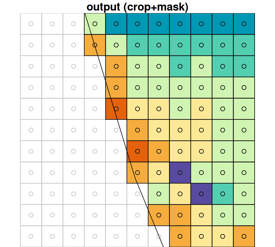
Figure 10.4: A small portion of the raster r_avg, brefore (left) after (right) cropping and masking
10.1.3 Masking-only
In case we need the output to keep the same extent as the input, we can mask a raster without cropping. Masking-only is done with the same operator ([), using the non-default argument crop=FALSE. To demonstrate the difference between masking+cropping (which we just did) and masking only, consider the following example where r_avg is masked and cropped (r_avg1), or just masked (r_avg2), according to the 'Negev' administrative area. First we prepare the polygon used for masking and cropping, obtained from a Shapefile named nafot.shp:
nafot = st_read('data/nafot.shp', quiet = TRUE)
nafot = st_transform(nafot, st_crs(r))
pol = nafot[nafot$name_eng == "Be'er Sheva", ]
Then we produce the masked+cropped (r_avg1) and masked (r_avg2) rasters:
As we can see in Figure 10.5, masking transforms pixel values to NA (both panels) while cropping also reduces raster extent by deleting whole rows and columns (left panel).
plot(r_avg1, key.pos = NULL, reset = FALSE, breaks = 'equal', col = hcl.colors(11, 'Spectral'), main = 'crop=TRUE (default)')
plot(st_geometry(pol), add = TRUE)
plot(st_as_sfc(st_bbox(r_avg1)), border = 'grey', add = TRUE)
plot(r_avg2, key.pos = NULL, reset = FALSE, breaks = 'equal', col = hcl.colors(11, 'Spectral'), main = 'crop=FALSE')
plot(st_geometry(pol), add = TRUE)
plot(st_as_sfc(st_bbox(r_avg2)), border = 'grey', add = TRUE)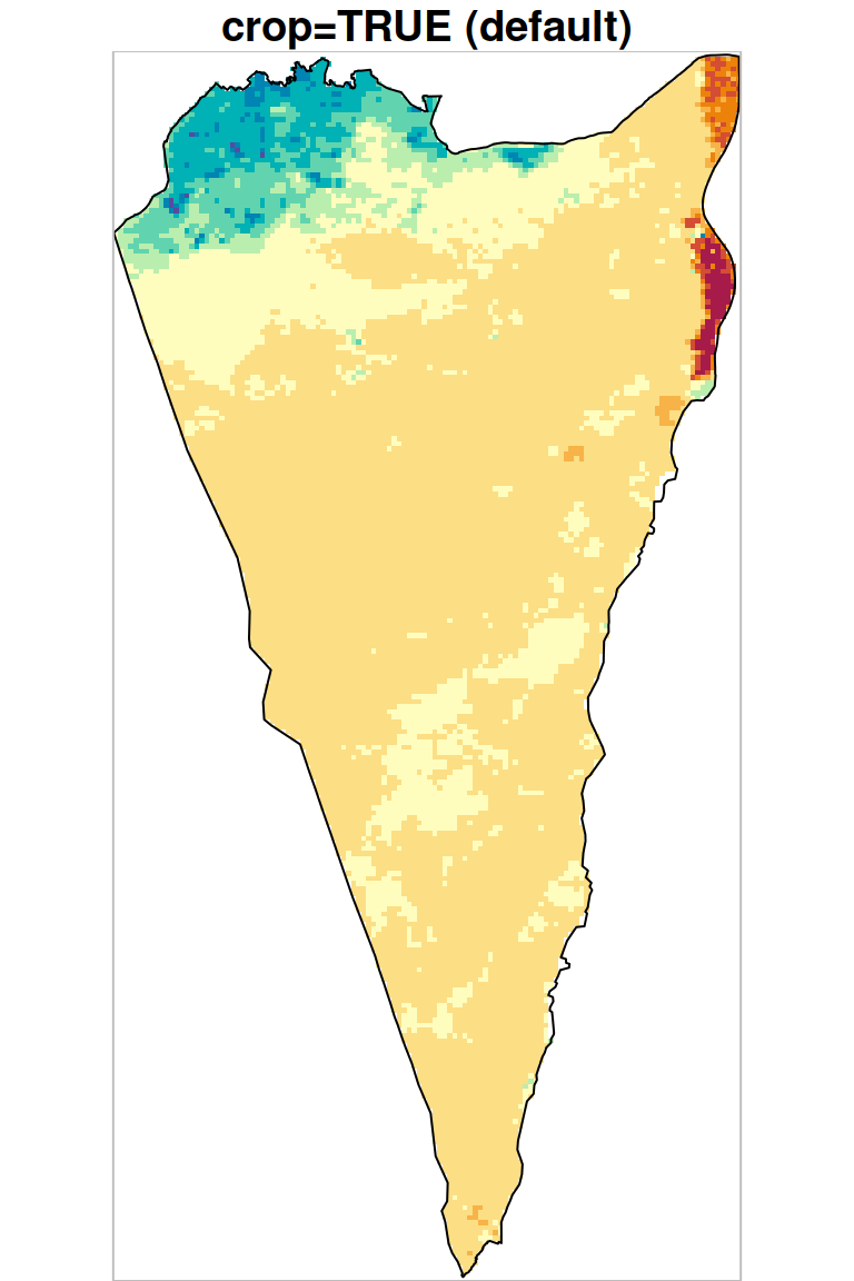
Figure 10.5: Cropping and masking (left) vs. masking (right), raster extent is shown in grey
Note that for plotting the raster extents (grey boxes in Figure 10.5), the above code section uses a combination of st_bbox and st_as_sfc. The combination returns the bounding box of a stars (or sf) layer as an sfc (geometry) object. For example, the following expression returns a geometry column with a single polygon, which is the bounding box of r_avg1:
10.2 Vector layer → raster
10.2.1 The st_rasterize function
The st_rasterize function converts a vector layer to a raster, given two arguments:
sf—The vector layer to converttemplate—A raster ‘template’ (if missing, it can be generated automatically)
The resulting raster retains the original values, from the template, in pixels that do not overlap with the vector layer (Figure 10.6). For pixels that do overlap with the vector layer, the value of the (first) vector layer attribute is “burned” into the pixels. The default meaning of the term “overlap” in the context of point, line, or polygon geometries, is:
- Pixels that a point intersects with
- Pixels chosen using Bresenham’s line algorithm
- Pixels whose centroid intersects with the polygon
The additional parameter options="ALL_TOUCHED=TRUE" can be passed to st_rasterize so that all pixels intersecting with the geometry are considered “overlapping” (Figure 10.6).
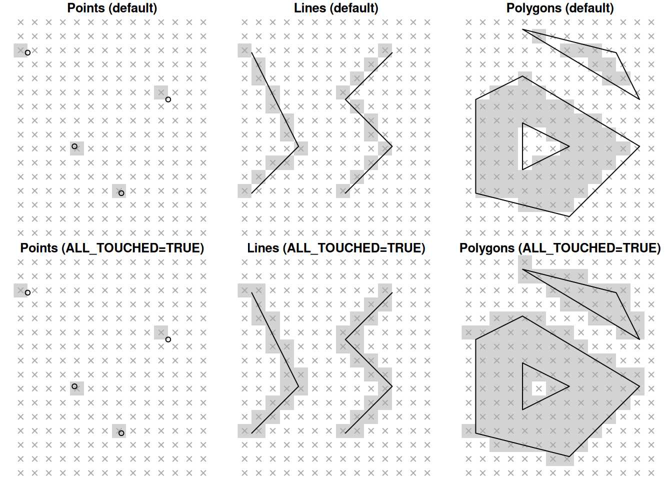
Figure 10.6: Rasterizing points, lines and polygons to raster with st_rasterize, using the default algorithms (top) and options="ALL_TOUCHED=TRUE" (bottom).
By default, the values are burned sequentially, according to the order of features. Therefore, when there are more than one vector features coinciding with the same pixel, the attribute value of the last feature “wins”. Alternatively, we can add up all values of coinciding geometries, using the argument options="MERGE_ALG=ADD" (Section 10.2.3).
10.2.2 Rasterizing polygon attributes
For an example of rasterizing a polygon layer, let’s convert the nafot vector layer to a raster, using r_avg as the template. The attribute which will be “burned” into the raster is the Id of the administrative area:
The resulting raster s has the same dimensions of r_avg but different values, as shown in Figure 10.7. We can see that those areas not covered by the nafot layer retained their original value (average NDVI). All pixels that were covered by nafot got the Id attribute value.
plot(nafot[, 'Id'], col = NA, main = "nafot[, 'Id']", border = NA, reset = FALSE, key.pos = NULL, axes = TRUE)
plot(nafot[, 'Id'], key.pos = NULL, add = TRUE)
plot(nafot[, 'Id'], col = NA, main = NA, border = NA, reset = FALSE, key.pos = NULL, axes = TRUE)
plot(r_avg, breaks = 'equal', main = 'r_avg', add = TRUE)
plot(nafot[, 'Id'], col = NA, main = NA, border = NA, reset = FALSE, key.pos = NULL, axes = TRUE)
plot(s, breaks = 'equal', col = sf.colors(nrow(nafot)), main = "st_rasterize(nafot[, 'Id'], r_avg)", add = TRUE)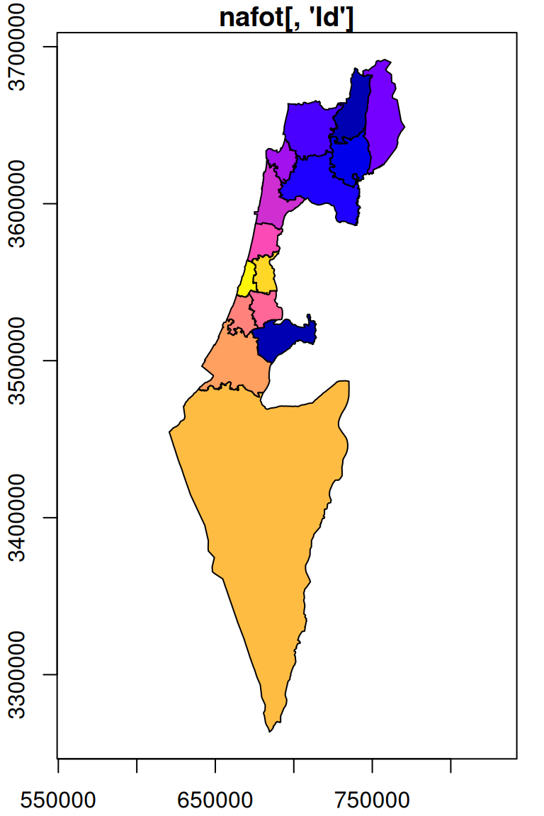
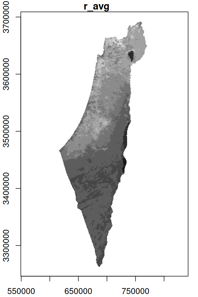
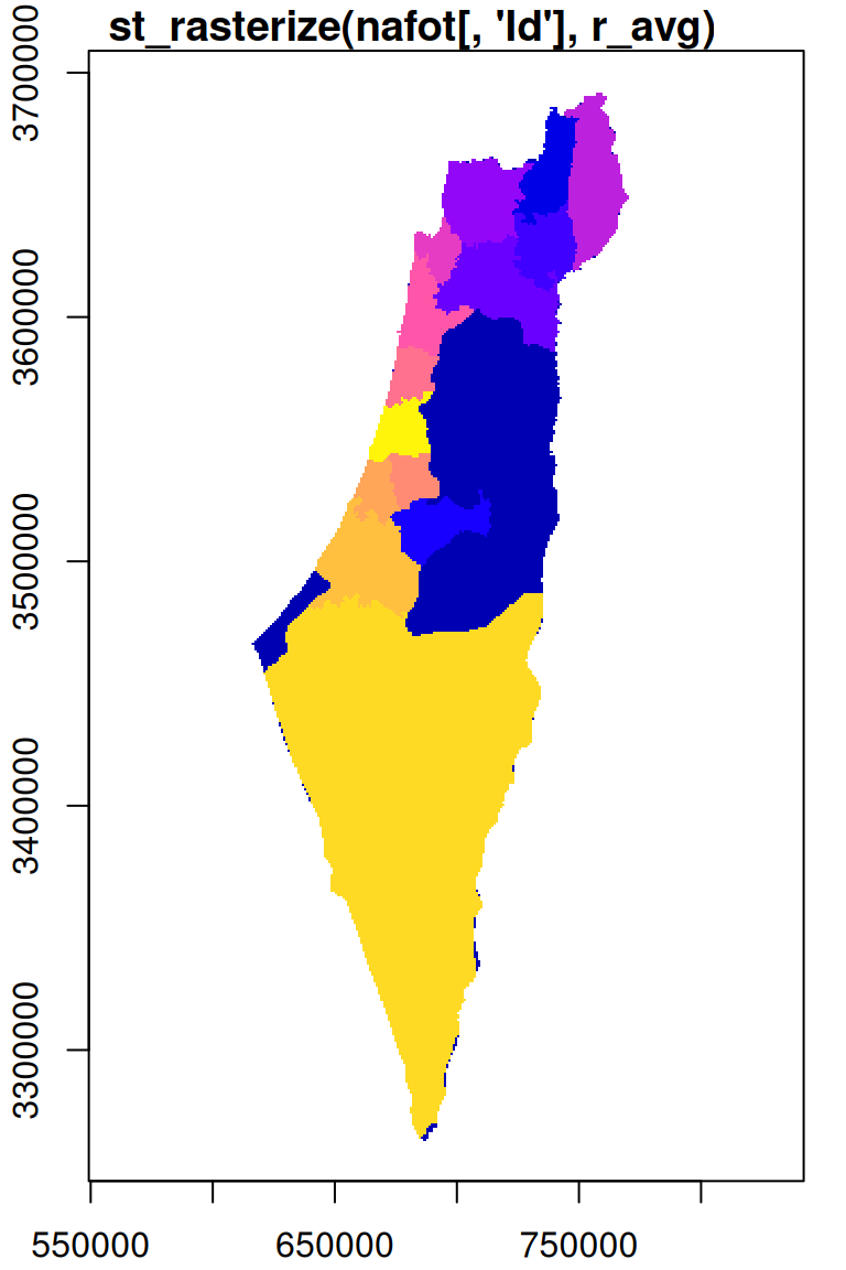
Figure 10.7: Rasterizing the Id of the nafot administrative areas layer into the average NDVI raster
Instead of retaining the original values, typically we want to start with an empty template, so that the only values in the resulting raster are those coming from the vector layer. For example, we can use a copy of the r_avg raster, where all of the pixel values are replaced with NA, as the template:
The result is shown in Figure 10.8:
plot(nafot[, 'Id'], main = "nafot[, 'Id']", key.pos = NULL, axes = TRUE)
plot(nafot[, 'Id'], col = NA, main = 'template', border = NA, reset = FALSE, key.pos = NULL, axes = TRUE)
plot(nafot[, 'Id'], col = NA, main = NA, border = NA, reset = FALSE, key.pos = NULL, axes = TRUE)
plot(s, breaks = 'equal', col = sf.colors(nrow(nafot)), main = "st_rasterize(nafot[, 'Id'], template)", add = TRUE)
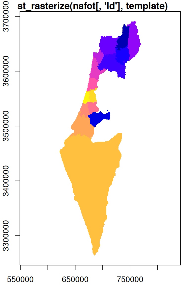
Figure 10.8: Rasterizing into an empty template
Keep in mind that only numeric attributes can be rasterized. Trying to rasterize a vector layer with one non-numeric attribute results in default sequential ID values rasterized instead. Rasterizing a vector layer with more than one (numeric) attribute will result in a stars object with several attributes.
10.2.3 Rasterizing point counts
Sometimes we want to add up attribute values from overlapping features coinciding with the same pixel, rather than take the last value. This is useful, for instance, when calculating a point density raster. For example, let’s read the plants.shp and reserve.shp Shapefiles. These Shapefiles contain a point layer of rare plants observations and a polygon with the borders of Negev Mountains Nature Reserve, the largest nature reserve in Israel, respectively:
plants = st_read('data/plants.shp', quiet = TRUE)
reserve = st_read('data/reserve.shp', quiet = TRUE)
We will also reproject both layers to UTM, so that all pixels correspond to equal area size, which is more appropriate for density calculations:
Figure 10.9 shows both layers—the polygonal layer reserve and the point layer plants:
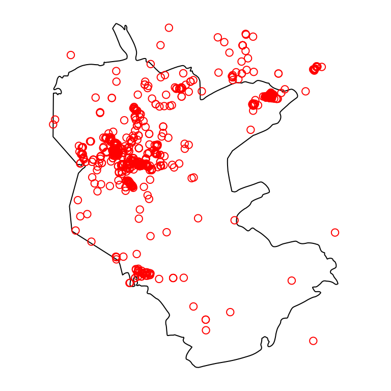
Figure 10.9: Nature reserve and rare plants observations
How can we calculate a raster expressing the density of plants points across the nature reserve? First, we set up an empty template raster, where all pixels within the area of interest—the nature reserve—are given an initial value of zero, using st_as_stars (Section 9.2.1):
template = st_as_stars(st_bbox(reserve), dx = 2000, dy = 2000)
template[[1]][] = 0
template = template[reserve]
Figure 10.10 shows the template:
plot(template, text_values = TRUE, breaks = 'equal', col = 'lightgrey', reset = FALSE)
plot(st_geometry(reserve), add = TRUE)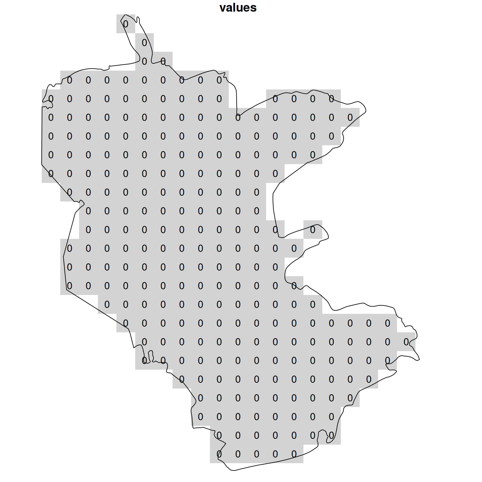
Figure 10.10: Template for calculating point density
Then, we create a new attrubute named count, with a value of 1 for each plant observation:
Finally, we rasterize the 'count' attribute into the template raster, with an additional option options='MERGE_ALG=ADD' (Section 10.2.1). The 'MERGE_ALG=ADD' option acts as a flag instructing st_rasterize to add up any overlapping attributes “burned” into the same pixel:
The resulting raster values reflect the sum of the count attribute from all overlapping points per pixel, i.e., the number of rare plant observations per pixel (Figure 10.11):
plot(s, text_values = TRUE, breaks = 'equal', col = function(n) hcl.colors(n, 'Reds', rev = TRUE), reset = FALSE)
plot(st_geometry(reserve), add = TRUE)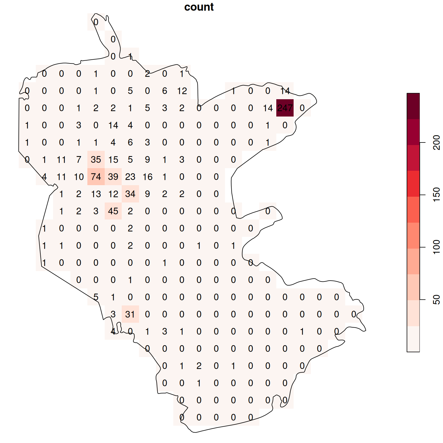
Figure 10.11: Density (observations per pixel) of rare plants in the nature reserve
The raster coloring is almost uniform, because the distribution is highly skewed. Namely, there are a lot of pixels with zero count, and few pixels with high count (try running hist(s[[1]]) to see that). We can use a logarithmic color scale to visualize the density pattern more clearly (Figure 10.12). Now we can see which parts of the reserve were characterized by higher occurence of rare plants.
b = c(0, 10^(seq(0, log10(max(s[[1]], na.rm=TRUE))+0.1, 0.1)))
plot(s, text_values = TRUE, breaks = b, reset = FALSE, col = hcl.colors(length(b)-1, 'Reds', rev = TRUE))
plot(st_geometry(reserve), add = TRUE)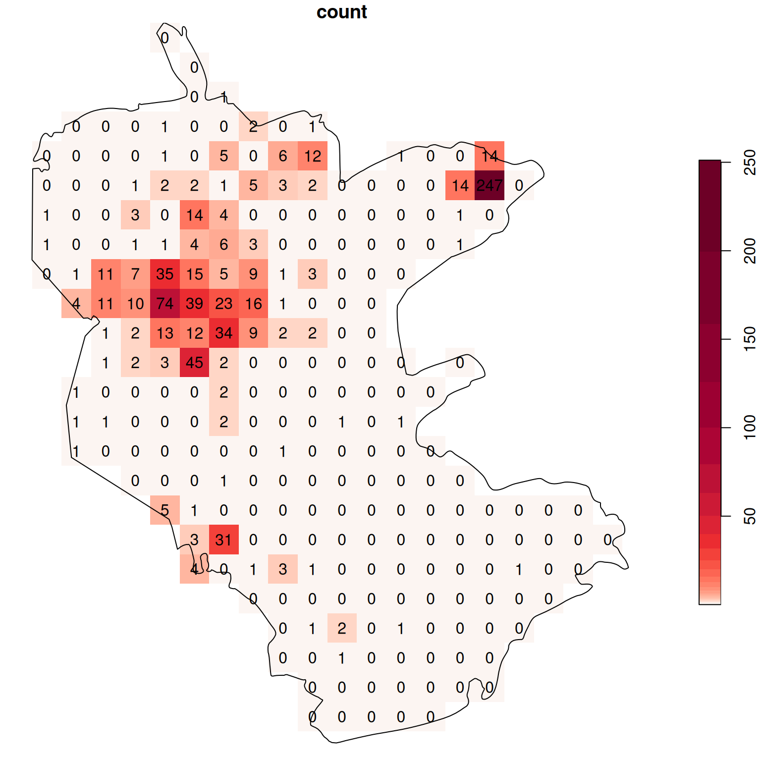
Figure 10.12: Density (observations per pixel) of rare plants in the nature reserve, with a logarithmic color scale
10.2.4 Standardizing density units
In the observation density raster s (Section 10.2.3), the units of measurement are plants per pixel. Since a pixel happens to have an area of 4 \(km^2\) (see below), raster values are, in fact, counts per 4 \(km^2\).
We know that the area of a pixel is 4 \(km^2\) since we set the resolution to 2000 \(m\) (Section 10.2.3). In general, however, we can apply the st_area function to calculate pixel area sizes of any raster. Recall that, when applied on a vector layer, st_area returns a vectot of units values, with the corresponding areas of all geometries (Section 8.3.2.2). When st_area is applied on a raster, it returns a raster of area values per pixel:
a = st_area(s)
a
## stars object with 2 dimensions and 1 attribute
## attribute(s):
##             Min. 1st Qu. Median  Mean 3rd Qu.  Max.
## area [m^2] 4e+06   4e+06  4e+06 4e+06   4e+06 4e+06
## dimension(s):
##   from to  offset delta                refsys point x/y
## x    1 21  645913  2000 WGS 84 / UTM zone 36N FALSE [x]
## y    1 25 3394893 -2000 WGS 84 / UTM zone 36N FALSE [y]
As usual, the area values are given in CRS units (in this case, \(m^2\)). We can transform the matrix with the entire raster values (a[[1]]) from \(m^2\) to \(km^2\) units, using set_units (Section 8.3.2.2):
library(units)
a[[1]] = set_units(a[[1]], 'km^2')
a
## stars object with 2 dimensions and 1 attribute
## attribute(s):
##             Min. 1st Qu. Median Mean 3rd Qu. Max.
## area [km^2]    4       4      4    4       4    4
## dimension(s):
##   from to  offset delta                refsys point x/y
## x    1 21  645913  2000 WGS 84 / UTM zone 36N FALSE [x]
## y    1 25 3394893 -2000 WGS 84 / UTM zone 36N FALSE [y]
Finally, we can examine one of the raster values. It doesn’t matter which one, since all pixels have exactly the same area. For example, the following expression gives the top-left corner value from the stars values matrix:
Let’s return to the density raster s. It is more convenient to work with counts per standard area unit, such as plants per 1 \(km^2\). To do that, we can divide the plants count raster s, by pixel area raster a:
The result is a raster with counts per unit area, in this case plant observations per \(km^2\):
s
## stars object with 2 dimensions and 1 attribute
## attribute(s):
##                  Min. 1st Qu. Median     Mean 3rd Qu.  Max. NA's
## density [1/km^2]    0       0      0 0.804902    0.25 61.75  270
## dimension(s):
##   from to  offset delta                refsys point x/y
## x    1 21  645913  2000 WGS 84 / UTM zone 36N FALSE [x]
## y    1 25 3394893 -2000 WGS 84 / UTM zone 36N FALSE [y]
The result is shown in Figure 10.13:
b = c(0, 10^(seq(0, log10(as.numeric(max(s[[1]], na.rm=TRUE)))+0.1, 0.1)))
plot(round(s, 1), text_values = TRUE, breaks = b, reset = FALSE, col = hcl.colors(length(b)-1, 'Reds', rev = TRUE))
plot(st_geometry(reserve), add = TRUE)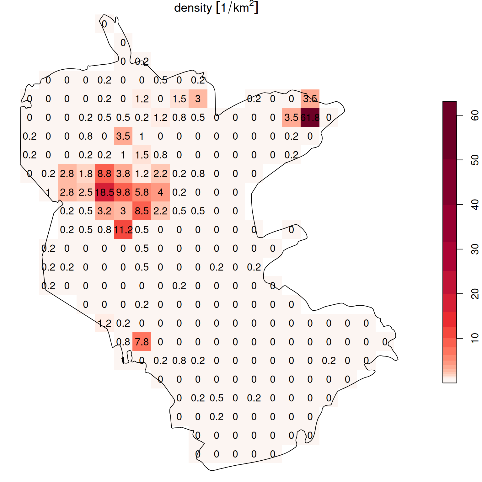
Figure 10.13: Density (observations per \(km^2\)) of rare plants in the nature reserve, with a logarithmic scale
We now move on to the opposite operation, converting a raster to a vector layer. As we will see, there are three variants of this conversion:
10.3 Raster → Polygons
10.3.1 Raster to polygons conversion
The st_as_sf function makes the raster to polygons conversion, when using the (default) as_points=FALSE argument. Furthermore:
The
st_as_sffunction ignores pixels that haveNAvalues in all layers. If necessary, we can convert those pixels that haveNAin all layers to polygons, too, by specifyingna.rm=FALSE.A useful option
merge=TRUEdissolves all adjacent polygons that have the same raster value (in the first layer) into a single feature. The dissolve algorithm can be specified with theconnect8parameter: 4d, which is the default (connect8=FALSE) or 8d (connect8=TRUE).
The attribute table of the polygon layer that we create contains the raster values—with a separate attribute for each raster band.
For example, let’s take a small subset of the raster r:
We will replace some of the pixel values with NA:
and round the values to one digit:
The resulting small raster u is visualized in Figure 10.14. Note that the raster has one pixel with NA in both layers, and another pixel with NA in the first layer only.
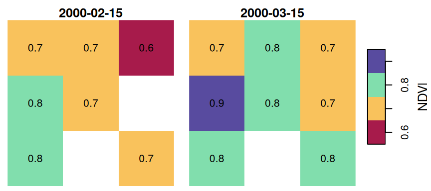
Figure 10.14: Sample raster
Now, let’s try using st_as_sf to transform the small raster u to a polygon layer p:
The resulting polygonal layer p has eight polygons, even though the raster u had nine pixels. This is because one of the pixels had NA in all layers, and therefore it was not converted to a polygon:
p
## Simple feature collection with 8 features and 2 fields
## Geometry type: POLYGON
## Dimension:     XY
## Bounding box:  xmin: 727089 ymin: 3610119 xmax: 729867.9 ymax: 3612898
## Projected CRS: WGS 84 / UTM zone 36N
##   2000-02-15 2000-03-15                       geometry
## 1        0.7        0.7 POLYGON ((727089 3612898, 7...
## 2        0.7        0.8 POLYGON ((728015.3 3612898,...
## 3        0.6        0.7 POLYGON ((728941.6 3612898,...
## 4        0.8        0.9 POLYGON ((727089 3611972, 7...
## 5        0.7        0.8 POLYGON ((728015.3 3611972,...
## 6         NA        0.7 POLYGON ((728941.6 3611972,...
## 7        0.8        0.8 POLYGON ((727089 3611046, 7...
## 8        0.7        0.8 POLYGON ((728941.6 3611046,...
The resulting layer p, which has eight features and two attributes, is shown in Figure 10.15:
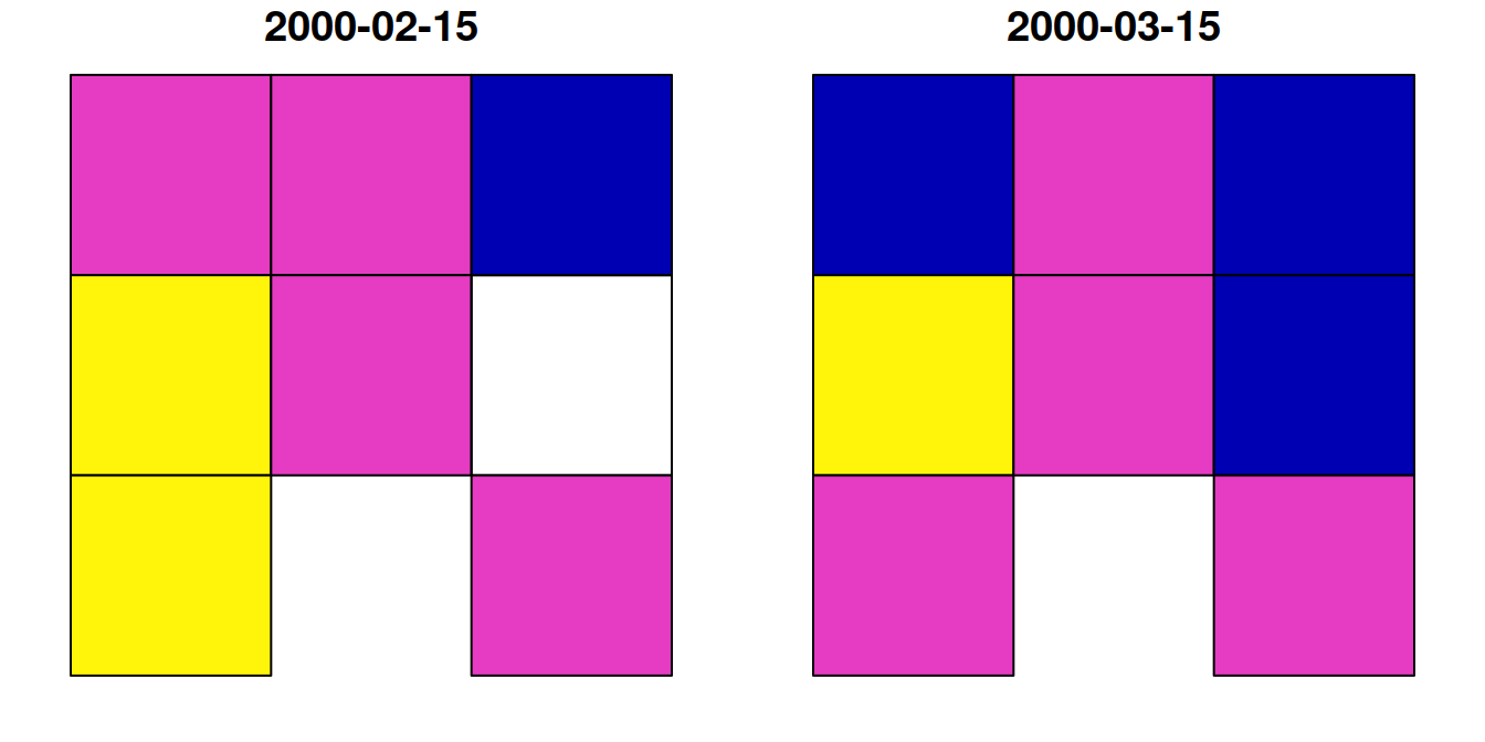
Figure 10.15: Polygon layer created from a raster
Compare this with st_as_sf(..., na.rm=FALSE), which retains all pixels:
st_as_sf(u, na.rm = FALSE)
## Simple feature collection with 9 features and 2 fields
## Geometry type: POLYGON
## Dimension:     XY
## Bounding box:  xmin: 727089 ymin: 3610119 xmax: 729867.9 ymax: 3612898
## Projected CRS: WGS 84 / UTM zone 36N
##   2000-02-15 2000-03-15                       geometry
## 1        0.7        0.7 POLYGON ((727089 3612898, 7...
## 2        0.7        0.8 POLYGON ((728015.3 3612898,...
## 3        0.6        0.7 POLYGON ((728941.6 3612898,...
## 4        0.8        0.9 POLYGON ((727089 3611972, 7...
## 5        0.7        0.8 POLYGON ((728015.3 3611972,...
## 6         NA        0.7 POLYGON ((728941.6 3611972,...
## 7        0.8        0.8 POLYGON ((727089 3611046, 7...
## 8         NA         NA POLYGON ((728015.3 3611046,...
## 9        0.7        0.8 POLYGON ((728941.6 3611046,...
Now, let’s try the merge=TRUE option. Since merging only retains the first raster band, we must convert each band to a separate polygon layer:
As a result, we have two separate polygonal layers p1 and p2:
p1
## Simple feature collection with 4 features and 1 field
## Geometry type: POLYGON
## Dimension:     XY
## Bounding box:  xmin: 727089 ymin: 3610119 xmax: 729867.9 ymax: 3612898
## Projected CRS: WGS 84 / UTM zone 36N
##   NDVI                       geometry
## 1  0.6 POLYGON ((728941.6 3612898,...
## 2  0.7 POLYGON ((727089 3612898, 7...
## 3  0.8 POLYGON ((727089 3611972, 7...
## 4  0.7 POLYGON ((728941.6 3611046,...
p2
## Simple feature collection with 6 features and 1 field
## Geometry type: POLYGON
## Dimension: XY
## Bounding box: xmin: 727089 ymin: 3610119 xmax: 729867.9 ymax: 3612898
## Projected CRS: WGS 84 / UTM zone 36N
## NDVI geometry
## 1 0.7 POLYGON ((727089 3612898, 7...
## 2 0.8 POLYGON ((728015.3 3612898,...
## 3 0.7 POLYGON ((728941.6 3612898,...
## 4 0.9 POLYGON ((727089 3611972, 7...
## 5 0.8 POLYGON ((727089 3611046, 7...
## 6 0.8 POLYGON ((728941.6 3611046,...Figure 10.16 displays both p1 and p2:
plot(p1, main = paste0('p1 (', nrow(p1), ' features)'))
plot(p2, main = paste0('p2 (', nrow(p2), ' features)'))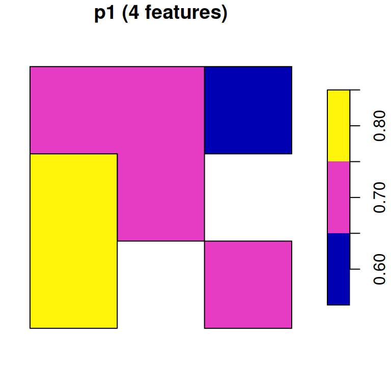
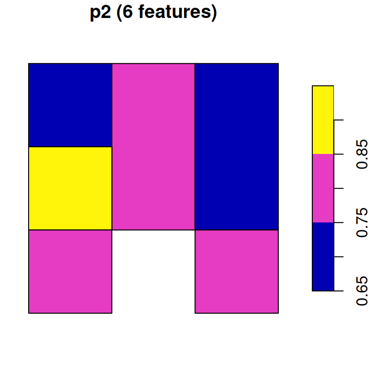
Figure 10.16: Polygon layer created from a raster
Do you think there will there be a difference, in terms of the number of features in
p1and inp2, if we useconnect8=TRUE? Re-runst_as_sfwithconnect8=TRUEto check your answer.
10.3.2 Segmentation
One example of a use case of raster to polygon conversion is the delineation of distinct inter-connected groups of pixels, sharing the same (or a similar) value. This operation is also known as segmentation. In its simplest form—detecting segments with exactly the same value—segmentation can be done using st_as_sf with merge=TRUE.
For example, we can derive segments of NDVI>0.2 in the reclassified NDVI raster l_rec_focal from Section 9.4.3. First, let’s recreate the l_rec_focal raster:
l = read_stars('data/landsat_04_10_2000.tif')
red = l[,,,3,drop=TRUE]
nir = l[,,,4,drop=TRUE]
ndvi = (nir - red) / (nir + red)
names(ndvi) = 'NDVI'
l_rec = ndvi
l_rec[l_rec < 0.2] = 0
l_rec[l_rec >= 0.2] = 1
get_neighbors = function(m, pos) {
  i = (pos[1]-1):(pos[1]+1)
  j = (pos[2]-1):(pos[2]+1)
  as.vector(t(m[i, j]))
}
focal2 = function(r, fun, ...) {
  template = r
  input = t(template[[1]])
  output = matrix(NA, nrow = nrow(input), ncol = ncol(input))
  for(i in 2:(nrow(input) - 1)) {
    for(j in 2:(ncol(input) - 1)) {
      v = get_neighbors(input, c(i, j))
      output[i, j] = fun(v, ...)
    }
  }
  template[[1]] = t(output)
  return(template)
}
l_rec_focal = focal2(l_rec, max)
Segments in the l_rec_focal raster represent distinct continuous areas with \(NDVI>0.2\). To detect them, we can convert the raster to polygons using st_as_sf with the merge=TRUE:
Then, we filter only those segments where raster value was 1:
The result is a polygon layer where each feature represents a single continuous area where \(NDVI>0.2\):
pol
## Simple feature collection with 536 features and 1 field
## Geometry type: POLYGON
## Dimension:     XY
## Bounding box:  xmin: 663975 ymin: 3459405 xmax: 687645 ymax: 3488145
## Projected CRS: WGS 84 / UTM zone 36N
## First 10 features:
##    NDVI                       geometry
## 3     1 POLYGON ((675615 3488145, 6...
## 4     1 POLYGON ((676455 3488145, 6...
## 6     1 POLYGON ((684765 3488145, 6...
## 8     1 POLYGON ((681945 3488145, 6...
## 12    1 POLYGON ((687195 3488145, 6...
## 13    1 POLYGON ((686985 3488085, 6...
## 20    1 POLYGON ((686505 3488145, 6...
## 25    1 POLYGON ((665865 3488145, 6...
## 26    1 POLYGON ((685545 3488145, 6...
## 27    1 POLYGON ((686835 3487905, 6...
Figure 10.17 shows the segments on top of the NDVI raster:
plot(ndvi, breaks = 'equal', col = hcl.colors(11, 'Spectral'), reset = FALSE, key.pos = 4)
plot(st_geometry(pol), add = TRUE)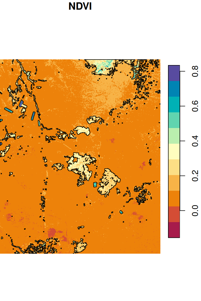
Figure 10.17: Segments with NDVI>0.2
What is the exact number of segments in
pol? If we ran thest_as_sffunction onl_recinstead ofl_rec_focal, do you think the number of segments would be higher or lower?
10.4 Raster → Points
The Raster→Points transformation is done using function st_as_sf with the as_points=TRUE option. Pixel centers—except for pixels with NA in all layers—become points. Just like in a conversion to polygons (Section 10.3), the attribute table of the resulting point layer contains the raster values.
For example, here is how we can transform the small raster u to a point layer:
p = st_as_sf(u, as_points = TRUE)
p
## Simple feature collection with 8 features and 2 fields
## Geometry type: POINT
## Dimension:     XY
## Bounding box:  xmin: 727552.1 ymin: 3610583 xmax: 729404.8 ymax: 3612435
## Projected CRS: WGS 84 / UTM zone 36N
##   2000-02-15 2000-03-15                 geometry
## 1        0.7        0.7 POINT (727552.1 3612435)
## 2        0.7        0.8 POINT (728478.4 3612435)
## 3        0.6        0.7 POINT (729404.8 3612435)
## 4        0.8        0.9 POINT (727552.1 3611509)
## 5        0.7        0.8 POINT (728478.4 3611509)
## 6         NA        0.7 POINT (729404.8 3611509)
## 7        0.8        0.8 POINT (727552.1 3610583)
## 8        0.7        0.8 POINT (729404.8 3610583)
The point layer p is shown in Figure 10.18:
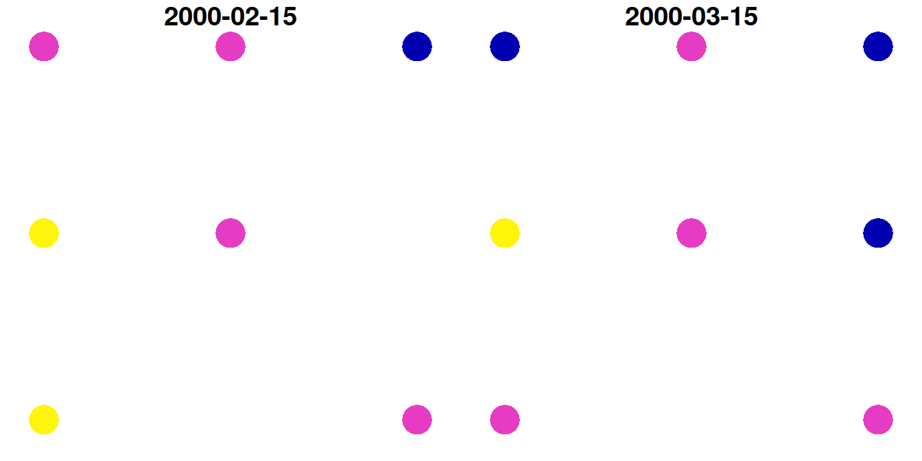
Figure 10.18: Point layer created from a raster
Same as in the polygons example (Section 10.3), the resulting point layer p has eight features, even though the raster had nine pixels, because one of the pixels had NA in all layers and therefore was not converted to a point. Again, if necessary, we can keep the pixels that have NA in all layers by specifying na.rm=FALSE:
st_as_sf(u, as_points = TRUE, na.rm = FALSE)
## Simple feature collection with 9 features and 2 fields
## Geometry type: POINT
## Dimension:     XY
## Bounding box:  xmin: 727552.1 ymin: 3610583 xmax: 729404.8 ymax: 3612435
## Projected CRS: WGS 84 / UTM zone 36N
##   2000-02-15 2000-03-15                 geometry
## 1        0.7        0.7 POINT (727552.1 3612435)
## 2        0.7        0.8 POINT (728478.4 3612435)
## 3        0.6        0.7 POINT (729404.8 3612435)
## 4        0.8        0.9 POINT (727552.1 3611509)
## 5        0.7        0.8 POINT (728478.4 3611509)
## 6         NA        0.7 POINT (729404.8 3611509)
## 7        0.8        0.8 POINT (727552.1 3610583)
## 8         NA         NA POINT (728478.4 3610583)
## 9        0.7        0.8 POINT (729404.8 3610583)
10.5 Distance to nearest point
Another example of a spatial operator involving a raster and a vector layer is the calculation of a raster of distances to the nearest point. For example, we may be interested in mapping the distances to the nearest meteorological stations in Israel, to evaluate where coverage is too sparse and reliable meteorological data are missing.
We are already familiar with the st_distance function for calculating distances (Section 8.3.2.3). However, st_distance expects two vector layers as input, not a vector layer and a raster. Therefore, to calculate a raster of distances from nearest point, we first need to convert the “template” raster to a point layer (Section 10.4). In this example, our template for the distances raster, hereby named grid, is the \(926\times926\) \(m^2\) raster r_avg (though we could use any other raster template). The NDVI attribute is discarded, since it is irrelevant for the distance calculation:
grid = st_as_sf(r_avg, as_points = TRUE)
grid$NDVI = NULL
grid
## Simple feature collection with 32858 features and 0 fields
## Geometry type: POINT
## Dimension:     XY
## Bounding box:  xmin: 616395.6 ymin: 3262292 xmax: 770162.2 ymax: 3692097
## Projected CRS: WGS 84 / UTM zone 36N
## First 10 features:
##                    geometry
## 1  POINT (757193.9 3691171)
## 2  POINT (758120.2 3691171)
## 3  POINT (759046.5 3691171)
## 4  POINT (753488.7 3690245)
## 5    POINT (754415 3690245)
## 6  POINT (755341.3 3690245)
## 7  POINT (756267.6 3690245)
## 8  POINT (757193.9 3690245)
## 9  POINT (758120.2 3690245)
## 10 POINT (759046.5 3690245)
Let’s also import the point layer of meteorological stations (Section 7.4):
rainfall = read.csv('data/rainfall.csv')
rainfall = st_as_sf(rainfall, coords = c('x_utm', 'y_utm'), crs = 32636)
Now we can use st_distance to calculate pairwise distances between every grid point (grid) and meteorological station (rainfall):
The result d is a distance matrix. Its rows correspond to grid points and its columns correspond to rainfall points. This is a very large matrix, due to the large number of grid points:
In this example, we are interested in the minimal distance, per grid point, among the distances to the 169 meteorological stations. Therefore we apply the min function on the distance matrix rows (Section 4.5), which refer to grid points. The result is a numeric vector of minimal distances, which we assign as an attribute in grid:
It is also convenient to convert the distances from from \(m\) to \(km\). Since apply returns numeric, thus “losing” the units of measurement, we first need to convert the distances to units and only then make the conversion:
The grid point layer now has an attribute named dist, with the distance to nearest meteorological station, in \(km\):
grid
## Simple feature collection with 32858 features and 1 field
## Geometry type: POINT
## Dimension:     XY
## Bounding box:  xmin: 616395.6 ymin: 3262292 xmax: 770162.2 ymax: 3692097
## Projected CRS: WGS 84 / UTM zone 36N
## First 10 features:
##                    geometry          dist
## 1  POINT (757193.9 3691171) 15.72760 [km]
## 2  POINT (758120.2 3691171) 16.40858 [km]
## 3  POINT (759046.5 3691171) 17.11260 [km]
## 4  POINT (753488.7 3690245) 12.55666 [km]
## 5    POINT (754415 3690245) 13.14112 [km]
## 6  POINT (755341.3 3690245) 13.76317 [km]
## 7  POINT (756267.6 3690245) 14.41792 [km]
## 8  POINT (757193.9 3690245) 15.10113 [km]
## 9  POINT (758120.2 3690245) 15.80911 [km]
## 10 POINT (759046.5 3690245) 16.53868 [km]
The result is shown in Figure 10.19:
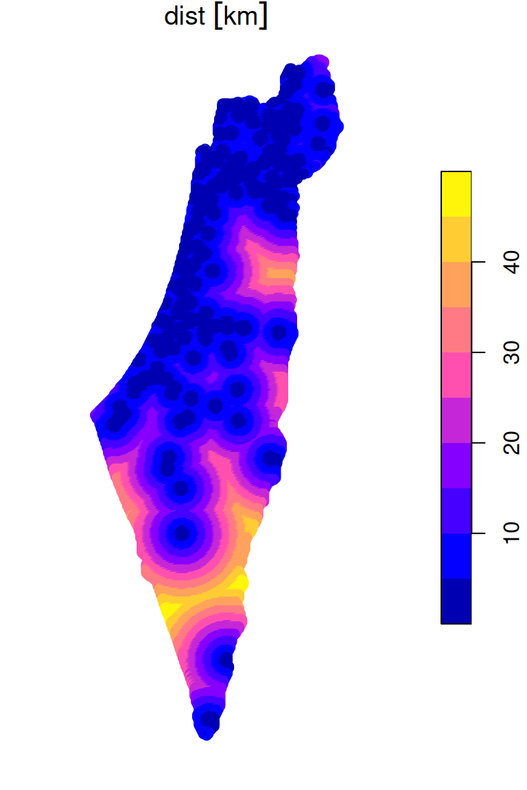
Figure 10.19: Distance to nearest meteorological station (point grid)
To have the results back as a raster, we can rasterize the points (Section 10.2). We should use the same raster which we started with to create the points—this guarantees that every point corresponds exactly to one pixel:
The final raster with distances to the nearest stations is shown in Figure 10.20. The locations of the meteorological stations and contour lines are shown on top of the raster, to emphasize the distance gradient:
plot(distance, breaks = 'equal', col = terrain.colors(10), reset = FALSE)
plot(st_geometry(rainfall), add = TRUE, pch = 3, cex = 0.4)
contour(distance, add = TRUE)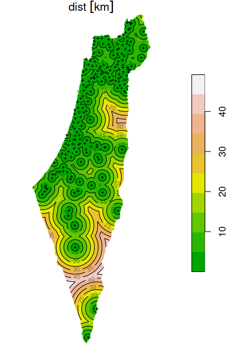
Figure 10.20: Distance to nearest meteorological station (raster)
10.6 Raster → Lines (contours)
We already saw how a raster can be converted to polygons (Section 10.3) or to points (Section 10.4), which simply results in a layer of cell outlines or centroids, respectively. Another common transformation is to calculate contour lines of equal raster values.
To illustrate contour lines calculation, we will reconstruct the Haifa DEM at 90 \(m\) resolution (Section 9.3):
dem1 = read_stars('data/srtm_43_06.tif')
dem2 = read_stars('data/srtm_44_06.tif')
dem = st_mosaic(dem1, dem2)
names(dem) = 'elevation'
dem = dem[, 5687:6287, 2348:2948]
dem = st_warp(src = dem, crs = 32636, cellsize = 90)
Raster contours can be calculated using the st_contour function. The function can accept a breaks argument, which determines the break points where contours are generated. Another parameter named contour_lines determines whether contours are returned as a line layer (TRUE) or polygon layer (FALSE, the default).
To decide on breaks values we are interested in, it is useful to examine the range of values in the raster:
According to the above result, we will use breaks from -100 to 600 meters, in steps of 50 meters:
The result, dem_contour, is a LINESTRING layer with one feature per contour line:
dem_contour
## Simple feature collection with 612 features and 1 field
## Geometry type: LINESTRING
## Dimension:     XY
## Bounding box:  xmin: 678607.1 ymin: 3602252 xmax: 710107.1 ymax: 3658412
## Projected CRS: WGS 84 / UTM zone 36N
## First 10 features:
##    elevation                       geometry
## 1        150 LINESTRING (704500.1 365832...
## 2        150 LINESTRING (704680.1 365832...
## 3        200 LINESTRING (707113.3 365841...
## 4        100 LINESTRING (701332.1 365823...
## 5        350 LINESTRING (708883.5 365841...
## 6        150 LINESTRING (706102.1 365802...
## 7        100 LINESTRING (702198.3 365823...
## 8         50 LINESTRING (700342.1 365746...
## 9        200 LINESTRING (704932.1 365719...
## 10       450 LINESTRING (709117.1 365728...
The contours are shown in Figure 10.21:
plot(dem, breaks = b, col = terrain.colors(length(b)-1), key.pos = 4, reset = FALSE)
plot(st_geometry(dem_contour), add = TRUE)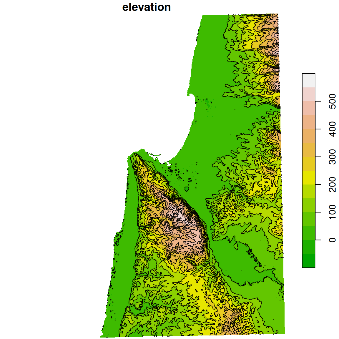
Figure 10.21: Contour lines
10.7 Extracting raster values
10.7.1 Introduction
It is often necessary to “extract” raster values according to overlapping vector features, such as points, lines or polygons (Figure 10.22). For example, given an NDVI raster, we may be interested in calculating the NDVI value observed in particular point locations, or the average NDVI observed over an administrative area polygon.

Figure 10.22: Extracting raster values (http://rpubs.com/etiennebr/visualraster)
When extracting values to lines or polygons, it is common to summarize the values that the geometry intersects with, using a function such as mean. That way, the values can “fit” into a new attribute, or several attributes. Extracting to points is simpler, because each geometry corresponds to one pixel, so there is nothing to summarize.
Extracting to points can be accompished with the st_extract function, while extracting to lines or to polygons can be accomplished with the aggregate function. In the next few sections, we will see examples of the most common extract scenarios:
10.7.2 Extracting to points: single-band
10.7.2.1 NDVI in meteorological stations
Raster values can be extracted to points using the st_extract function. The function accepts:
x—astarsrasterpts—asfpoint layer
and returns a new sf layer, with an additional attribute containing the values from x from the matching pixel for each point in pts.
For example, we can determine the average NDVI (r_avg) in the pixel where each meteorological station (rainfall) falls in, as follows:
x = st_extract(r_avg, rainfall)
x
## Simple feature collection with 169 features and 1 field
## Geometry type: POINT
## Dimension:     XY
## Bounding box:  xmin: 629301.4 ymin: 3270290 xmax: 761589.2 ymax: 3681163
## Projected CRS: WGS 84 / UTM zone 36N
## First 10 features:
##         NDVI                 geometry
## 1  0.4357747 POINT (696533.1 3660837)
## 2  0.3544532 POINT (697119.1 3656748)
## 3  0.3196541 POINT (696509.3 3652434)
## 4  0.4238691 POINT (696541.7 3641332)
## 5  0.3745760 POINT (697875.3 3630156)
## 6         NA POINT (687006.2 3633330)
## 7  0.4580601 POINT (689553.7 3626282)
## 8  0.3732974 POINT (694694.5 3624388)
## 9  0.5153764 POINT (686489.5 3619716)
## 10 0.4521039 POINT (683148.4 3616846)
The extracted values can be attached to the rainfall layer, using assignment:
As a result, the rainfall layer now has an additional attribuite named NDVI:
rainfall
## Simple feature collection with 169 features and 13 fields
## Geometry type: POINT
## Dimension:     XY
## Bounding box:  xmin: 629301.4 ymin: 3270290 xmax: 761589.2 ymax: 3681163
## Projected CRS: WGS 84 / UTM zone 36N
## First 10 features:
##       num altitude sep oct nov dec jan feb mar apr may              name
## 1  110050       30 1.2  33  90 117 135 102  61  20 6.7 Kfar Rosh Hanikra
## 2  110351       35 2.3  34  86 121 144 106  62  23 4.5              Saar
## 3  110502       20 2.7  29  89 131 158 109  62  24 3.8             Evron
## 4  111001       10 2.9  32  91 137 152 113  61  21 4.8       Kfar Masrik
## 5  111650       25 1.0  27  78 128 136 108  59  21 4.7     Kfar Hamakabi
## 6  120202        5 1.5  27  80 127 136  95  49  19 2.7        Haifa Port
## 7  120630      450 1.9  36  93 161 166 128  71  21 4.9  Haifa University
## 8  120750       30 1.6  31  91 163 170 146  76  22 4.9             Yagur
## 9  120870      210 1.1  32  93 147 147 109  61  16 4.3        Nir Etzyon
## 10 121051       20 1.8  32  85 147 142 102  56  13 4.5         En Carmel
##                    geometry      NDVI
## 1  POINT (696533.1 3660837) 0.4357747
## 2  POINT (697119.1 3656748) 0.3544532
## 3  POINT (696509.3 3652434) 0.3196541
## 4  POINT (696541.7 3641332) 0.4238691
## 5  POINT (697875.3 3630156) 0.3745760
## 6  POINT (687006.2 3633330)        NA
## 7  POINT (689553.7 3626282) 0.4580601
## 8  POINT (694694.5 3624388) 0.3732974
## 9  POINT (686489.5 3619716) 0.5153764
## 10 POINT (683148.4 3616846) 0.4521039
The attribute values are shown as text labels in Figure 10.23:
plot(r_avg, breaks = 'equal', col = hcl.colors(11, 'Spectral'), reset = FALSE)
text(st_coordinates(rainfall), as.character(round(rainfall$NDVI, 2)), cex = 0.5)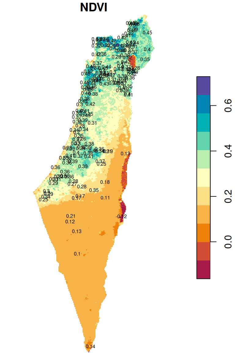
Figure 10.23: Raster values extracted to points
Now that we know the average NDVI for each meteorological station location, we can examine, for instance, the association between NDVI and rainfall in December (Figure 10.24):
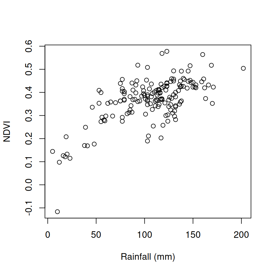
Figure 10.24: Average NDVI as function of average rainfall in December
What is the number and proportion of
rainfallpoints that have anNAvalue in theNDVIattribute? Why did those stations getNA?
10.7.3 Extracting to points: multi-band
As another example, we can extract the NDVI values for different dates from the multi-band raster r. For simplicity, let’s create a subset rainfall1, with just three meteorological stations from the rainfall layer:
sel = c('Horashim', 'Beer Sheva', 'Yotveta')
rainfall1 = rainfall[rainfall$name %in% sel, ]
rainfall1
## Simple feature collection with 3 features and 13 fields
## Geometry type: POINT
## Dimension:     XY
## Bounding box:  xmin: 671364.1 ymin: 3307819 xmax: 717491.2 ymax: 3648872
## Projected CRS: WGS 84 / UTM zone 36N
##        num altitude sep oct nov dec jan feb mar apr  may       name
## 77  212168      825 3.4  37 122 202 238 190 114  38 12.2   Horashim
## 141 251690      280 0.5   9  18  38  48  40  29   9  3.6 Beer Sheva
## 168 345005       80 0.4   2   2   6   5   4   5   2  0.4    Yotveta
##                     geometry      NDVI
## 77  POINT (717491.2 3648872) 0.5041712
## 141 POINT (671364.1 3458877) 0.1699691
## 168 POINT (700626.3 3307819)        NA
Now, let’s extract the NDVI values from a subset with the first five bands of r, into rainfall1:
This time, since extraction from a multi-band raster took place, the result is a stars object and not an sf object. Moreover, this is a special type of a stars object, with one dimension for the vector geometries (geometry) and another dimension for the raster layers (time):
rainfall1
## stars object with 2 dimensions and 1 attribute
## attribute(s):
##         Min. 1st Qu. Median      Mean  3rd Qu.   Max. NA's
## NDVI  0.1092 0.13005 0.1564 0.2613929 0.444225 0.5396    1
## dimension(s):
##          from to                refsys point
## geometry    1  3 WGS 84 / UTM zone 36N  TRUE
## time        1  5                  Date    NA
##                                                         values
## geometry POINT (717491.2 3648872),...,POINT (700626.3 3307819)
## time                                 2000-02-15,...,2000-06-15
To work with the data, it is often more convenient to transform this type of stars object to an sf layer. This can be done with st_as_sf:
rainfall1 = st_as_sf(rainfall1)
rainfall1
## Simple feature collection with 3 features and 5 fields
## Geometry type: POINT
## Dimension:     XY
## Bounding box:  xmin: 671364.1 ymin: 3307819 xmax: 717491.2 ymax: 3648872
## Projected CRS: WGS 84 / UTM zone 36N
##   2000-02-15 2000-03-15 2000-04-15 2000-05-15 2000-06-15
## 1     0.4314     0.4485     0.5396     0.5234     0.4772
## 2         NA     0.1587     0.1618     0.1541     0.1489
## 3     0.1440     0.1254     0.1251     0.1122     0.1092
##                   geometry
## 1 POINT (717491.2 3648872)
## 2 POINT (671364.1 3458877)
## 3 POINT (700626.3 3307819)
In case we are interested only in the extracted values, not the geometries, we can use st_drop_geometry:
rainfall1 = st_drop_geometry(rainfall1)
rainfall1
##   2000-02-15 2000-03-15 2000-04-15 2000-05-15 2000-06-15
## 1     0.4314     0.4485     0.5396     0.5234     0.4772
## 2         NA     0.1587     0.1618     0.1541     0.1489
## 3     0.1440     0.1254     0.1251     0.1122     0.1092
Finally, we can rely on the fact that row and column order matches the vector layer feature and raster layer order, respectively, to assign names. For example, rainfall1 rows correspond to the selected station names, therefore we can assign the station names into rownames:
rownames(rainfall1) = sel
rainfall1
##            2000-02-15 2000-03-15 2000-04-15 2000-05-15 2000-06-15
## Horashim       0.4314     0.4485     0.5396     0.5234     0.4772
## Beer Sheva         NA     0.1587     0.1618     0.1541     0.1489
## Yotveta        0.1440     0.1254     0.1251     0.1122     0.1092
Columns in
rainfall1are already named according to image dates. Where did these names come from?
The analogous operation in ArcGIS is the “Extract Multi Values to Points” tool (Figures 10.25–10.26).
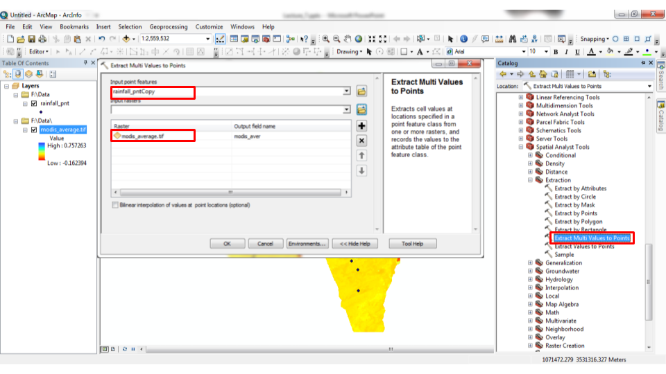
Figure 10.25: “Extract Multi Values to Points” tool in ArcGIS
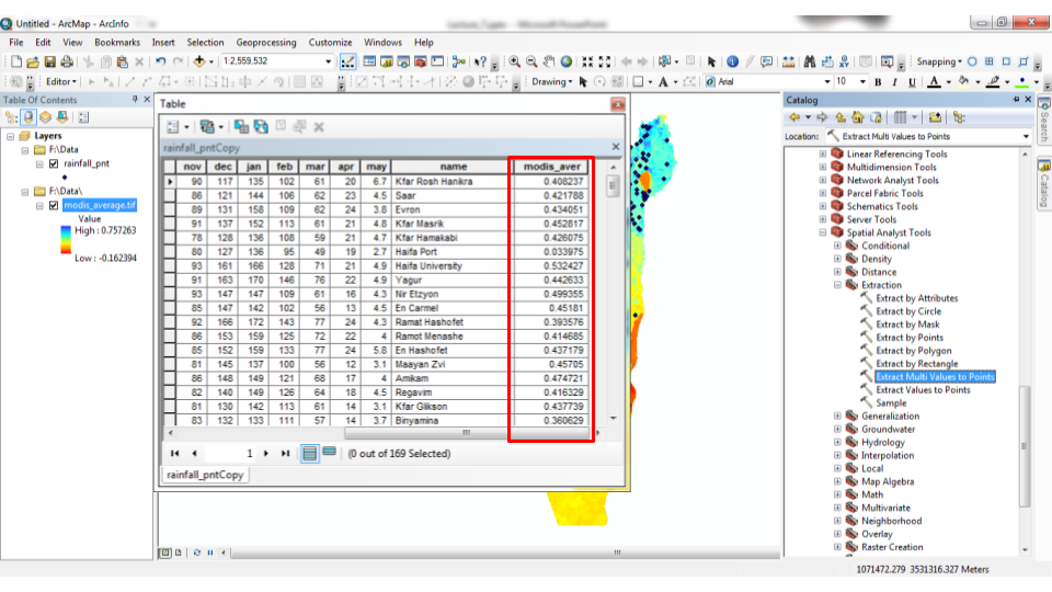
Figure 10.26: “Extract Multi Values to Points” tool in ArcGIS
10.7.4 Extracting to polygons: single-band
Extracting raster values to polygons (or to lines) is different from extracting to points. When extracting raster values to polygons (or to lines), each vector feature is potentially associated with more than one pixel value (Figure 10.22). Moreover, the number of pixels may vary between features. For example, a large polygon may cover many more pixels than a small polygon. Therefore, it is often convenient to summarize the raster values per polygon feauture by applying a function on them and obtaining a single number, such as the average. This is done by aggregating the raster based on a vector layer using function aggregate. (Recall that we already used aggregate for dissolving vector layers by attribute (Section 8.4).)
When summarizing raster values per polygon feature, the aggregate function accepts37:
x—Thestarsraster to summarizeby—Ansflayer determining areasFUN—The function to be applied on each set of extracted pixel values fromx
For example, we can calculate the average (mean) NDVI value (r_avg) per administrative area (nafot) as follows. Any additional arguments, such as na.rm=TRUE, are passed to the function, in this case so that mean excludes NA values:
The result is, again (Section 10.7.3), a special type of a stars object, with just one dimension for the vector geometries:
ndvi_nafot
## stars object with 1 dimensions and 1 attribute
## attribute(s):
##           Min.   1st Qu.    Median      Mean  3rd Qu.      Max.
## NDVI  0.126289 0.3375994 0.3845475 0.3553727 0.400052 0.4317472
## dimension(s):
##          from to                refsys point
## geometry    1 15 WGS 84 / UTM zone 36N FALSE
##                                                                 values
## geometry POLYGON ((739780.1 368600...,...,POLYGON ((674110.3 354916...
It can be converted to the more familiar sf structure using st_as_sf:
Now we have a polygon layer of the administrative areas, with an NDVI attribute containing the average NDVI value according to the r_avg raster:
ndvi_nafot
## Simple feature collection with 15 features and 1 field
## Geometry type: POLYGON
## Dimension:     XY
## Bounding box:  xmin: 620662.1 ymin: 3263494 xmax: 770624.4 ymax: 3691834
## Projected CRS: WGS 84 / UTM zone 36N
## First 10 features:
##         NDVI                       geometry
## 1  0.4208889 POLYGON ((739780.1 3686007,...
## 2  0.3845475 POLYGON ((672273.8 3518394,...
## 3  0.3093089 POLYGON ((745560 3649860, 7...
## 4  0.3874892 POLYGON ((702283.1 3628046,...
## 5  0.4317472 POLYGON ((702725.9 3630513,...
## 6  0.4051780 POLYGON ((759304.4 3691202,...
## 7  0.3949261 POLYGON ((701391.6 3631170,...
## 8  0.4124200 POLYGON ((706537.1 3602188,...
## 9  0.3937370 POLYGON ((692687.3 3583974,...
## 10 0.3468470 POLYGON ((672841.5 3544808,...
The result can be visualized as follows (Figure 10.27):
plot(ndvi_nafot, reset = FALSE, key.pos = 4)
text(st_coordinates(st_centroid(ndvi_nafot)), as.character(round(ndvi_nafot$NDVI, 2)))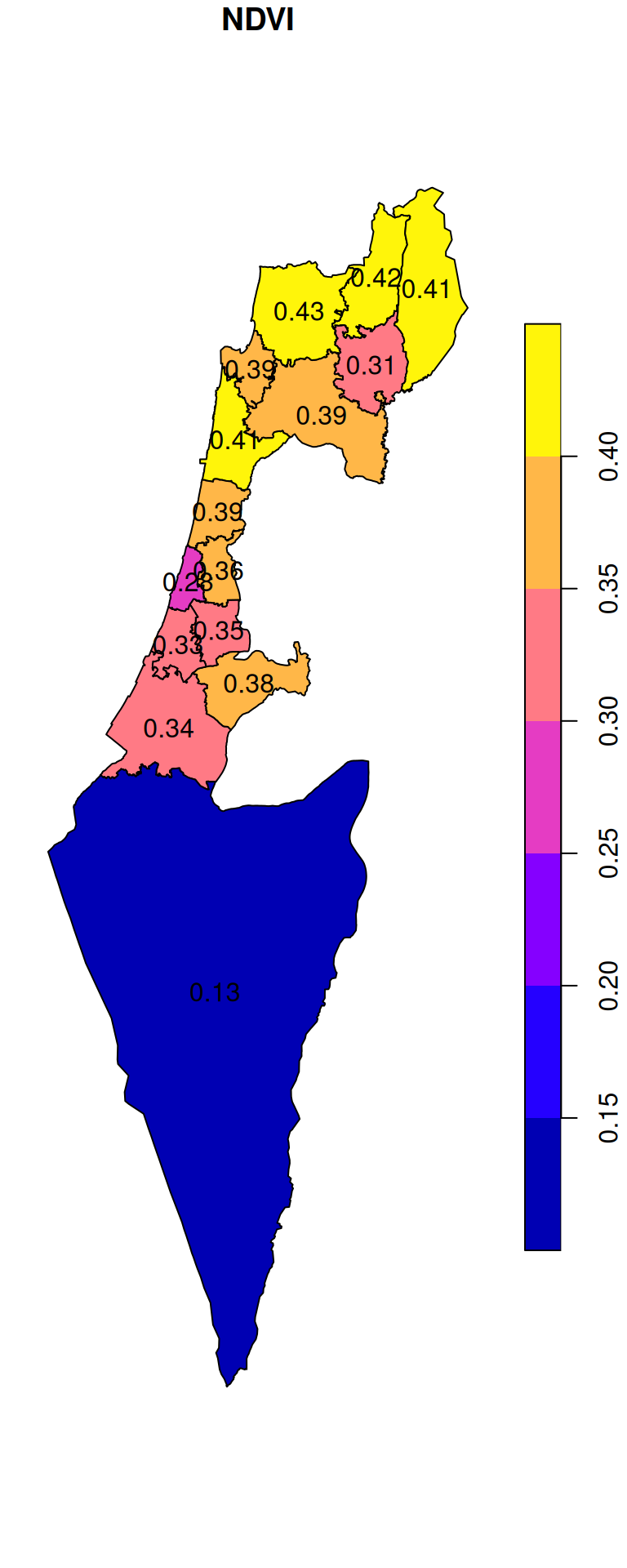
Figure 10.27: Average NDVI per “Nafa”
10.7.5 Extracting to polygons: multi-band
Extracting raster values from a multi-band raster works the same way as extracting from a multi-band raster. The difference is that the resulting stars object has two dimensions: one for the geometries and one for the input raster bands.
For example, the following expression calculates the average r value for each nafot feature over five months starting from 2000-02-01, based on the first five bands of r:
ndvi_nafot = aggregate(r[,,,1:5], nafot, mean, na.rm = TRUE)
ndvi_nafot
## stars object with 2 dimensions and 1 attribute
## attribute(s):
##            Min.   1st Qu.    Median      Mean   3rd Qu.      Max.
## NDVI  0.1082747 0.3147695 0.4407848 0.4023258 0.4872819 0.5905808
## dimension(s):
##          from to                refsys point
## geometry    1 15 WGS 84 / UTM zone 36N FALSE
## time        1  5                  Date    NA
##                                                                 values
## geometry POLYGON ((739780.1 368600...,...,POLYGON ((674110.3 354916...
## time                                         2000-02-15,...,2000-06-15
When transformed to an sf layer, the values extracted from each raster layer are placed in separate attributes:
ndvi_nafot = st_as_sf(ndvi_nafot)
ndvi_nafot
## Simple feature collection with 15 features and 5 fields
## Geometry type: POLYGON
## Dimension:     XY
## Bounding box:  xmin: 620662.1 ymin: 3263494 xmax: 770624.4 ymax: 3691834
## Projected CRS: WGS 84 / UTM zone 36N
## First 10 features:
##    2000-02-15 2000-03-15 2000-04-15 2000-05-15 2000-06-15
## 1   0.5061847  0.5270644  0.5319248  0.4432705  0.3478298
## 2   0.4692342  0.4604232  0.4568367  0.3757161  0.3096993
## 3   0.5395486  0.5398781  0.4491296  0.3011687  0.2440450
## 4   0.5616802  0.5826193  0.5475469  0.3978501  0.3062216
## 5   0.4718739  0.4840480  0.4993016  0.4304506  0.3796581
## 6   0.5518223  0.5851435  0.5905808  0.4905159  0.2675451
## 7   0.4593590  0.4520991  0.4388301  0.3730517  0.3468060
## 8   0.5061774  0.5087029  0.4809899  0.3971890  0.3509476
## 9   0.5104205  0.4970106  0.4763348  0.3797437  0.3421975
## 10  0.4709000  0.4675206  0.4407848  0.3536589  0.2844259
##                          geometry
## 1  POLYGON ((739780.1 3686007,...
## 2  POLYGON ((672273.8 3518394,...
## 3  POLYGON ((745560 3649860, 7...
## 4  POLYGON ((702283.1 3628046,...
## 5  POLYGON ((702725.9 3630513,...
## 6  POLYGON ((759304.4 3691202,...
## 7  POLYGON ((701391.6 3631170,...
## 8  POLYGON ((706537.1 3602188,...
## 9  POLYGON ((692687.3 3583974,...
## 10 POLYGON ((672841.5 3544808,...
The result reflects the average NDVI, for the first five months in the MODIS NDVI series, for each “Nafa” (Figure 10.28):
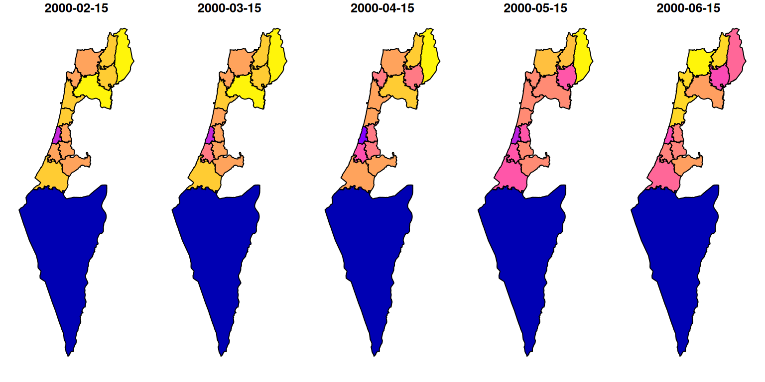
Figure 10.28: NDVI per “Nafa” for five months
Note that using
aggregateto extract raster values by polygons is only appropriate for non-overlapping polygons. For polygons that are potentially overlapping, useterra::extract.↩︎