Chapter 11 Processing spatio-temporal data

Last updated: 2024-03-20 11:49:33

Aims

Our aims in this chapter are:

• Learn to work with list objects
• Present several characteristics of spatio-temporal data
• Demonstrate spatio-temporal data processing:
  • Aggregation of raster spatio-temporal data
  • Reshaping of vector trajectory data

We will use the following R packages:

• stars
• dplyr
• data.table
• sf
• units

11.1 Lists

11.1.1 The list class

A list is a collection of objects of any class. There are no restrictions as for the class and dimensions of each list element. Lists are therefore the most flexible of the base R data structures.

A list can be created by passing individual objects to the list function. For example, the following expression creates a list object named x, which contains the three vectors c(1,3), c(4,5,6) and 8:

x = list(c(1, 3), c(4, 5, 6), 8)

Using the class function we can make sure that x is indeed a list:

class(x)
## [1] "list"

Printing a list shows the internal objects it contains. In an unnamed list, the elements are marked with indices inside double square brackets ([[):

x
## [[1]]
## [1] 1 3
## 
## [[2]]
## [1] 4 5 6
## 
## [[3]]
## [1] 8

List element names can be accessed with names:

names(x)
## NULL

and modified by assignment to names:

names(x) = c('a', 'b', 'c')

As a result of the above expression, x is now a named list. When printing a named list, elements are marked with $ symbols followed by element names:

x
## $a
## [1] 1 3
## 
## $b
## [1] 4 5 6
## 
## $c
## [1] 8

11.1.2 List subsetting

The [ operator gives a list subset, as a new list. Numeric indices, character indices (in case the list is named), or logical indices can be used. For example, either of the following expression returns a list with just the first two elements of x:

x[1:2]
## $a
## [1] 1 3
## 
## $b
## [1] 4 5 6

x[c('a', 'b')]
## $a
## [1] 1 3
## 
## $b
## [1] 4 5 6

Either of the following expressions returns a list with just the third element of x:

x[3]
## $c
## [1] 8

x['c']
## $c
## [1] 8

The [[ or $ operators return the contents of an individual list element (Figure 11.1). For example, either of the following expressions returns the second element of x, which is a numeric vector:

x[[2]]
## [1] 4 5 6

x[['b']]
## [1] 4 5 6

x$b
## [1] 4 5 6

Note that the [[ operator can be used with either numeric or character indices (in quotes), while the $ operator only works with character indices (without quotes).

Figure 11.1: The difference between the [ and [[ operators when subsetting a list (http://r4ds.had.co.nz/vectors.html)

List element names can be removed by assigning NULL to the names property:

names(x) = NULL

11.1.3 The lapply function

One of the most useful functions when working with list objects is lapply. The lapply function is used to “do something” with each list element, getting back a matching list of results. The lapply function:

• “Splits” a list to individual elements
• Calls a function on each element
• Combines the results back to a new list

The lapply function is therefore conceptually similar to apply (Section 4.5). The difference is that apply operates on rows or columns of a data.frame or matrix (Figure 11.2) (or rows/column/layer combinations of an array), while lapply operates on list elements.

Figure 11.2: apply and lapply

For example, the following expressions apply the mean (Figure 11.2), range and is.na functions on each element in the list x. In each case, the returned object from lapply a new list with the results:

lapply(x, mean)
## [[1]]
## [1] 2
## 
## [[2]]
## [1] 5
## 
## [[3]]
## [1] 8

lapply(x, range)
## [[1]]
## [1] 1 3
## 
## [[2]]
## [1] 4 6
## 
## [[3]]
## [1] 8 8

lapply(x, is.na)
## [[1]]
## [1] FALSE FALSE
## 
## [[2]]
## [1] FALSE FALSE FALSE
## 
## [[3]]
## [1] FALSE

11.1.4 The split function

The split function can be used to split a data.frame to a list of data.frame subsets, according to unique values of the given vector (Figure 11.3).

Figure 11.3: The split function

For the next example, let’s ctreate a small data.frame named dat:

dat = data.frame(
  y = c(3, 5, 1, 4, 5),
  g = c('f', 'm', 'f', 'f', 'm')
)
dat
##   y g
## 1 3 f
## 2 5 m
## 3 1 f
## 4 4 f
## 5 5 m

and a vector named a which matches the number of rows in dat:

a = c('a', 'a', 'b', 'a', 'b')
a
## [1] "a" "a" "b" "a" "b"

Using split, we can “split” dat to a list of subsets, with the corresponding rows to all levels in the vector a (Figure 11.3):

split(dat, a)
## $a
##   y g
## 1 3 f
## 2 5 m
## 4 4 f
## 
## $b
##   y g
## 3 1 f
## 5 5 m

Here is another example, using the small data.frame of railway stations from 4.1.2:

dat = data.frame(
    name = c('Beer-Sheva Center', 'Beer-Sheva University', 'Dimona'),
    city = c('Beer-Sheva', 'Beer-Sheva', 'Dimona'),
    lines = c(4, 5, 1),
    piano = c(FALSE, TRUE, FALSE)
)
dat
##                    name       city lines piano
## 1     Beer-Sheva Center Beer-Sheva     4 FALSE
## 2 Beer-Sheva University Beer-Sheva     5  TRUE
## 3                Dimona     Dimona     1 FALSE

Splitting by the 'city' column creates a list with two data.frame elements:

split(dat, dat$city)
## $`Beer-Sheva`
##                    name       city lines piano
## 1     Beer-Sheva Center Beer-Sheva     4 FALSE
## 2 Beer-Sheva University Beer-Sheva     5  TRUE
## 
## $Dimona
##     name   city lines piano
## 3 Dimona Dimona     1 FALSE

What will be the result of split(dat, dat$name)?

11.1.5 The do.call function

The do.call function can be used to pass a list of function arguments to another function. For example, instead of the following hypothetical function call of f with arguments a, b, c and d:

f(a, b, c, d)

we can use the following equivalent expression with do.call:

do.call(f, list(a, b, c, d))

The do.call function is useful when we want to call a function with a large or variable number of arguments—passed as list elements—without having to specify them by name.

For example, suppose we want to combine all internal vectors in the list x to a single vector, using the c function. Instead of specifying each and every element:

c(x[[1]], x[[2]], x[[3]])
## [1] 1 3 4 5 6 8

we can use do.call:

do.call(c, x)
## [1] 1 3 4 5 6 8

Now that we know how to work with list objects, we move on to defining spatio-temporal data (Section 11.2) and using the list class for spatio-temporal data processing (Sections 11.3–11.4).

11.2 Spatio-temporal data

It can be argued that all data are spatio-temporal, since they were measured in certain location(s) and time(s), even if the locations and times were not recorded and/or are irrelevant for analysis. However, we usually refer to data as spatio-temporal when the locations and times of observation were recorded and are relevant for analysis. Here are some examples of spatio-temporal data:

• Time-series of satellite images
• Temperature measurements in meteorological stations over time
• Voting results in administrative units during several election campaigns
• Movement tracks of people or animals, with or without associated measurements (heart rate, activity type, etc.)
• Spatial pattern of epidemic disease outbreak
• Volcanic eruption event locations over time

Methods and tools for processing and analyzing spatio-temporal data are generally less developed than methods for working with spatial or temporal data. R has numeroud specialized packages for analyzing spatio-temporal data. The important ones are listed in the Handling and Analyzing Spatio-Temporal Data task view.

Conceptually, we can classify types of spatio-temporal data according to the arrangement of observations in space-time (Figure 11.4). For example, spatio-temporal data may form a regular or irregular “grid”, depending on whether the observations were repeatedly measured at the same locations and times or whether each observations has a unique space-time “stamp”. Trajectories are distinguised by the fact that observations usually refer to an individual object (or few objects) observed in consecutive times.

Figure 11.4: Space-time dataset types (https://www.jstatsoft.org/article/view/v051i07)

For example, meteorological data (Figure 11.5) and satellite data (Figure 11.6) form regular grids of points or pixels collectively measured at the same time.

Figure 11.5: Grid layout: PM point measurements (https://edzer.github.io/UseR2016/)

Figure 11.6: Grid layout: Satellite image time series (Appel, Marius, and Edzer Pebesma. “On-Demand Processing of Data Cubes from Satellite Image Collections with the gdalcubes Library.” Data 4, no. 3 (2019): 92.)

Tweet (Figure 11.7) and disease case (Figure 11.8) locations comprise irregular grids, since each observation is associated with a unique location and timestamp.

Figure 11.7: Irregular layout: Tweets (http://onlinelibrary.wiley.com/doi/10.1111/j.1467-9671.2012.01359.x/abstract)

Figure 11.8: Irregular layout: Coral disease cases (http://journals.plos.org/plosone/article?id=10.1371/journal.pone.0004993)

Flickr image records per user over time (Figure 11.9) and storm tracks (Figure 11.10) are examples of trajectory data.

Figure 11.9: Trajectory: Flickr user paths

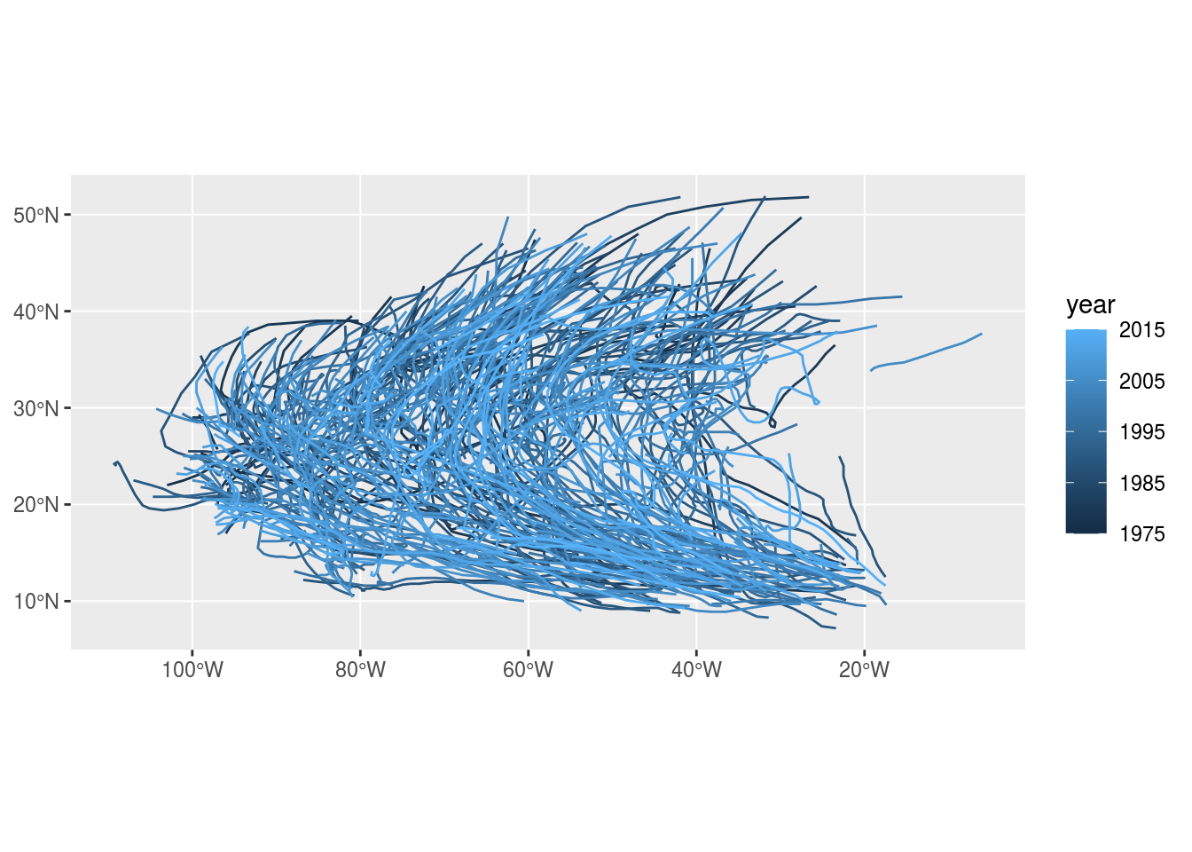
Figure 11.10: Trajectory: Storm paths (https://www.r-spatial.org/r/2017/08/28/nest.html)

11.3 Aggregation of spatio-temporal rasters

11.3.1 Introduction

Processing and visualization of spatio-temporal data are challenging, because of their three-dimensional nature. One of the basic approaches for working with spatio-temporal data is to simplify them using aggregation, in the spatial and/or temporal dimension, to help with visualization and exploratory analysis.

To demonstrate spatio-temporal aggregation, let’s go back to the MOD13A3_2000_2019.tif raster, which is an example of spatio-temporal data forming a regular grid (Figure 11.4):

library(stars)
r = read_stars('data/MOD13A3_2000_2019.tif')
dates = read.csv('data/MOD13A3_2000_2019_dates2.csv')
borders = st_read('data/israel_borders.shp', quiet = TRUE)
names(r) = 'NDVI'
dates$date = as.Date(dates$date)
r = st_set_dimensions(r, 'band', values = dates$date, names = 'time')
r = st_warp(r, crs = 32636)
r = r[borders]

11.3.2 Aggregating time periods

To aggregate a raster on the temporal dimension (the raster layer), we need to:

• Split the raster to subsets of raster layers (e.g., images captured in the different seasons)
• Use raster algebra to summarize each subset into a single layer (e.g., mean per pixel)
• Combine the results into a new multi-band raster (e.g., seasonal mean images)

We already learned how to subset raster layers using a numeric vector of indices (Section 6.2). Combined with which (Section 2.4.2), we can use this method to subset raster layers using a logical vector specifying which layers to keep. For example, here how we can get a subset of just the NDVI images taken in January:

r[,,,which(dates$month == 1)]
## stars object with 3 dimensions and 1 attribute
## attribute(s), summary of first 1e+05 cells:
##          Min. 1st Qu. Median      Mean 3rd Qu.   Max.  NA's
## NDVI  -0.1813   0.125 0.3528 0.3344972  0.4995 0.8861 60579
## dimension(s):
##      from  to  offset    delta                refsys
## x      80 246  542754  926.305 WGS 84 / UTM zone 36N
## y      14 478 3704603 -926.305 WGS 84 / UTM zone 36N
## time    1  19      NA       NA                  Date
##                                                   values x/y
## x                                                   NULL [x]
## y                                                   NULL [y]
## time [2001-01-15,2001-02-15),...,[2019-01-15,2019-02-15)

How can we create a subset of MOD13A3_2000_2019.tif with just the images taken during spring? How can we then calculate the “average” spring NDVI image?

Now, let’s use the same method to create a seasonal summary of average NDVI images, including each of the four seasons. We would like to create a raster named season_means, having 4 layers, where each layer is the average NDVI, excluding NA, per season:

• 'winter'
• 'spring'
• 'summer'
• 'fall'

First, we create a vector of season names:

seasons = c('winter', 'spring', 'summer', 'fall')

Then, iterating on the season names with a for loop, for each season we:

• Subset the layers captured in that season only
• Calculate the mean NDVI per pixel
• Collect the result into a list

The following code section initializes an empty list named season_means, then runs a for loop that goes over the seasons and calculates seasons means:

season_means = list()
for(i in seasons) {
  s = r[,,,which(dates$season == i)]
  season_means[[i]] = st_apply(s, c('x', 'y'), mean, na.rm = TRUE)
}

When the for loop ends, we get a list of seasonal mean rasters, named season_means.

(Note that passing a vector of indices does not work inside a for loop, which is why we are creating a vector named sel as an intermediate step. This is a bug in the current version of stars which is resolved in the development version.)

Next, we combine the list elements to a multi-band raster with do.call and c. The additional along=3 parameter makes sure the layers are “stacked” to form a third dimension:

season_means$along = 3
season_means = do.call(c, season_means)

This is basically a shortcut to the following alternative code, without using do.call, in which case we need to specify each and every one of the list items:

season_means = c(
  season_means[[1]],
  season_means[[2]],
  season_means[[3]],
  season_means[[4]],
  along = 3
)

Either way, we now have a four-band raster named season_mean with the seasonal means in r:

season_means
## stars object with 3 dimensions and 1 attribute
## attribute(s):
##          Min.   1st Qu.    Median      Mean   3rd Qu.   Max.   NA's
## mean  -0.1987 0.1107877 0.1786667 0.2311464 0.3325767 0.8181 179251
## dimension(s):
##         from  to  offset    delta                refsys          values x/y
## x         80 246  542754  926.305 WGS 84 / UTM zone 36N            NULL [x]
## y         14 478 3704603 -926.305 WGS 84 / UTM zone 36N            NULL [y]
## new_dim    1   4      NA       NA                    NA winter,...,fall

All we have left to do is set the attribute name ('NDVI') and dimension names:

names(season_means) = 'NDVI'
season_means = st_set_dimensions(season_means, names = c('x', 'y', 'season'))

Here is the modified season_means raster:

season_means
## stars object with 3 dimensions and 1 attribute
## attribute(s):
##          Min.   1st Qu.    Median      Mean   3rd Qu.   Max.   NA's
## NDVI  -0.1987 0.1107877 0.1786667 0.2311464 0.3325767 0.8181 179251
## dimension(s):
##        from  to  offset    delta                refsys          values x/y
## x        80 246  542754  926.305 WGS 84 / UTM zone 36N            NULL [x]
## y        14 478 3704603 -926.305 WGS 84 / UTM zone 36N            NULL [y]
## season    1   4      NA       NA                    NA winter,...,fall

Note that we do not need to set the layer dimention values, (i.e., the season names), since they are automatically populated with the names of the list elements in do.call.

The resulting season means raster is shown in Figure 11.11:

plot(season_means, breaks = 'equal', col = function(n) hcl.colors(n, 'Spectral'), key.pos = 4)

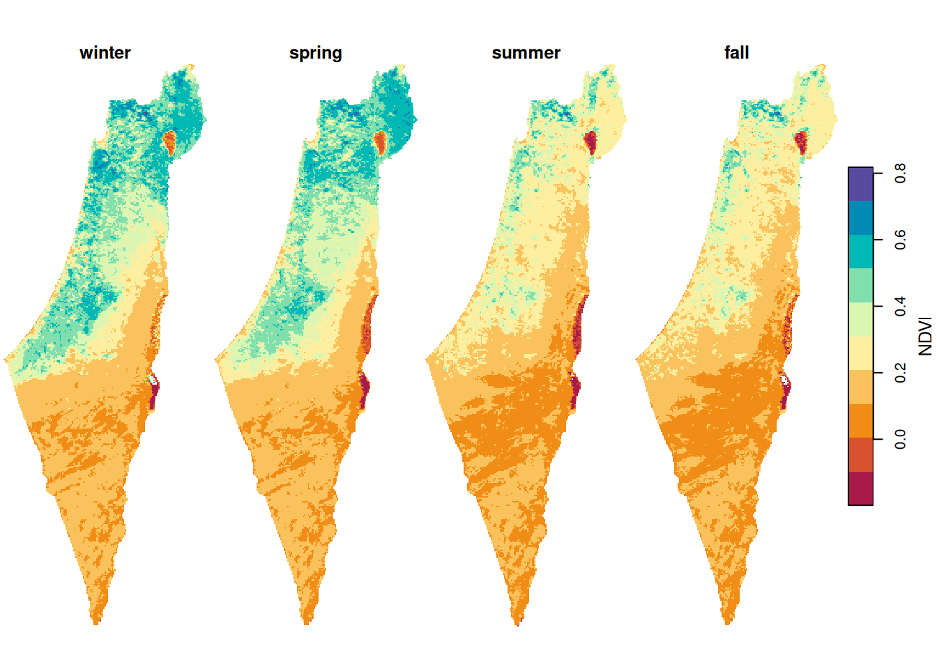
Figure 11.11: Average NDVI per season

In case we need to summarize the seasonal NDVI in a different way, all we have to do is replace the aggregation function. For example, we can decide to have NA instead of less reliable pixels where >10% of values are missing. In such case, instead of the previous function mean, we use a custom function named mean90:

mean90 = function(x) {if(mean(is.na(x)) > 0.1) NA else mean(x, na.rm = TRUE)}

The aggregation code are exactly the same as in the last example, except for using mean90—instead of mean—inside st_apply:

season_means = list()
for(i in seasons) {
  s = r[,,,which(dates$season == i)]
  season_means[[i]] = st_apply(s, c('x', 'y'), mean90)
}
season_means$along = 3
season_means = do.call(c, season_means)
names(season_means) = 'NDVI'
season_means = st_set_dimensions(season_means, names = c('x', 'y', 'season'))

The result is similar, only with some pixels replaced with NA:

plot(season_means, breaks = 'equal', col = function(n) hcl.colors(n, 'Spectral'), key.pos = 4)

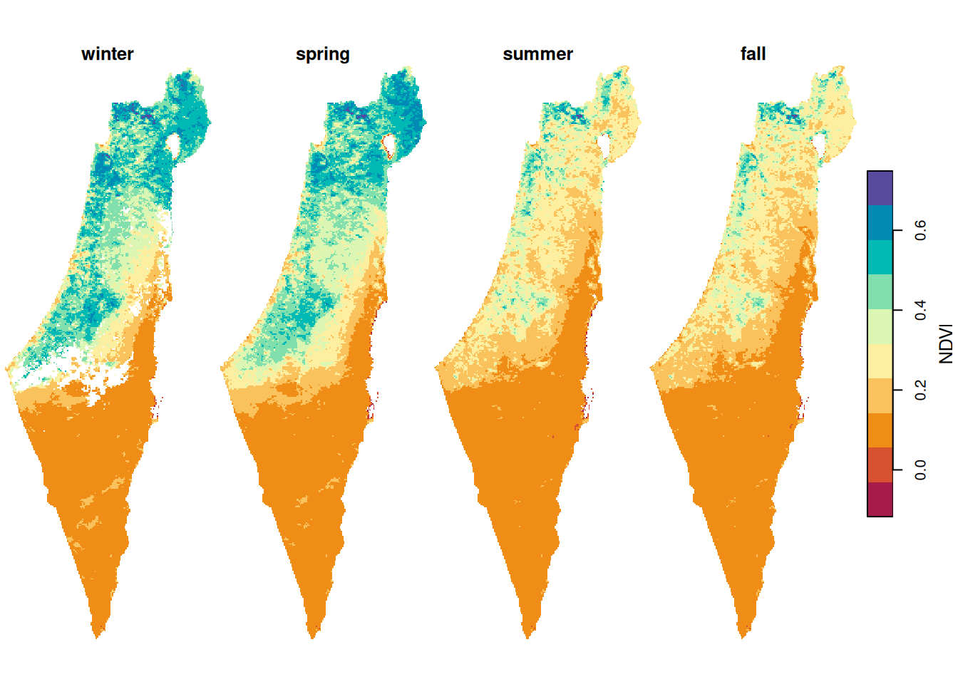
Figure 11.12: Average NDVI per season, pixels with >25% NA excluded

The pattern of NA values can be visualized by applying is.na on the result (Figure 11.13):

plot(is.na(season_means)[borders], col = c('grey90', 'red'))

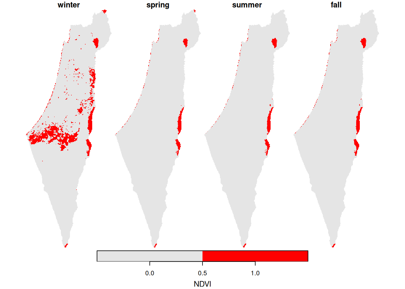
Figure 11.13: Location of pixels with >10% NA per season

What is the purpose of the [borders] part in the above expression? What happens without it?

11.3.3 Aggregating the 'x' dimension

Our second example demonstrates aggregation in one of the spatial dimensions, rather than in the layers dimension (Section 11.3.2). In this example, we will summarize the west-east gradient, i.e., the 'x' dimension or raster columns, into a single value. That way, we will be able to visualize how NDVI changes acrosss the remaining spatial dimension 'y', i.e., the north-south gradient, and over time.

First, let’s aggregate the 'x' dimension for specific points in time, to visualize the north-south NDVI gradient during two time points only. This can be done by applying the mean function on all rows for particular layers, such as layers 1 and 7:

x = st_apply(r[,,,1], 'y', mean, na.rm = TRUE)[[1]]   # Winter
y = st_apply(r[,,,7], 'y', mean, na.rm = TRUE)[[1]]   # Summer

The resulting vectors can be plotted as follows (Figure 11.14):

plot(x, type = 'l', col = 'blue', xlab = 'Row', ylab = 'NDVI')
lines(y, col = 'red')

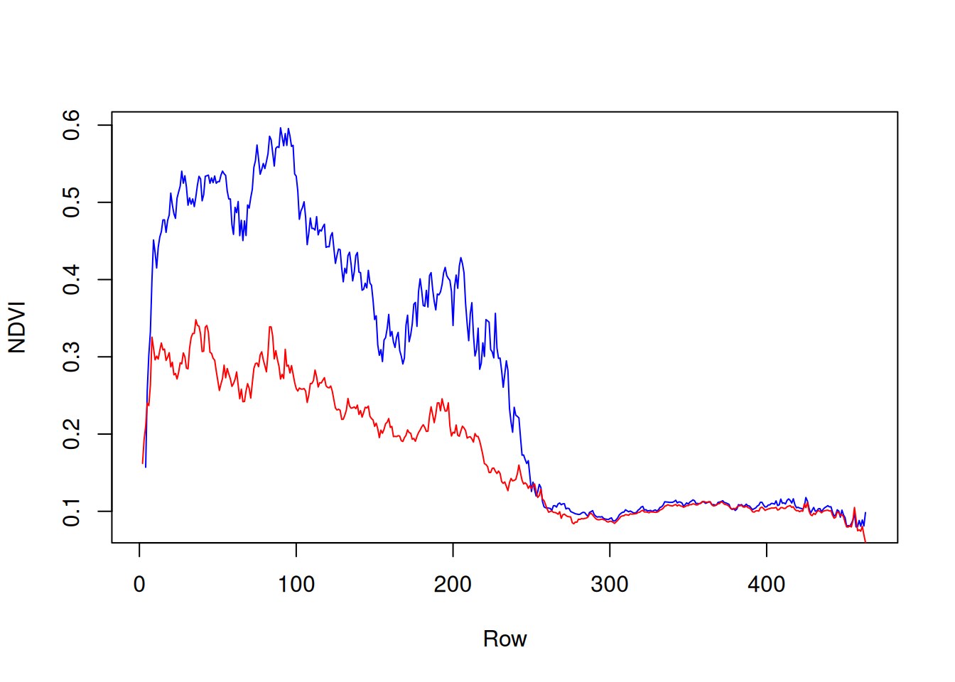
Figure 11.14: North-south NDVI gradient in two different months: February 2000 (blue) and August 2000 (red)

Now we are going to repeat the operation for all layers of r, rather than two specific layers 1 and 7. In other words, we will calculate the north-south gradient for all time points (layers) in the raster r. We will create a raster s, where each column will contain the row means of one layer of r (Figure 11.15).

Figure 11.15: Raster row means

Raster s is going to have:

• The same number of rows as r, i.e., 167 rows
• As many columns as r layers, i.e., 233 columns

To create s, we aggregate on dimensions 'y' and 'time', so that we calculate the mean of each 'y' and 'time' combination, i.e., each row. Consequently, all values along 'x' are averaged:

s = st_apply(r, c('y', 'time'), mean, na.rm = TRUE)
names(s) = 'NDVI'

The resulting stars object s has two dimensions, 'y' and 'time', and its values are the average NDVI values for entire rows:

s
## stars object with 2 dimensions and 1 attribute
## attribute(s):
##          Min.  1st Qu.    Median     Mean   3rd Qu.      Max. NA's
## NDVI  -0.1011 0.109609 0.1948469 0.229913 0.3214095 0.7447308  733
## dimension(s):
##      from  to  offset    delta                refsys                    values
## y      14 478 3704603 -926.305 WGS 84 / UTM zone 36N                      NULL
## time    1 233      NA       NA                  Date 2000-02-15,...,2019-06-15

The arrangement of s is very convenient in case we want to work with the data as a matrix or as a data.frame. For example, transforming s to a data.frame results in a table where the NDVI value in each y and time combination is in a separate row:

dat = as.data.frame(s)
head(dat)
##         y       time      NDVI
## 1 3692561 2000-02-15       NaN
## 2 3691634 2000-02-15       NaN
## 3 3690708 2000-02-15       NaN
## 4 3689782 2000-02-15 0.1570333
## 5 3688855 2000-02-15 0.2565000
## 6 3687929 2000-02-15 0.3022000

However, the s object does not have “spatial” x-y dimensions, which means that—strictly speaking—s is not a spatial raster. Therefore, it can’t be simply displayed with plot:

plot(s)
## Error in plot.stars(s): no raster, no features geometries: no default plot method set up yet!

In order to visualize s, we can modify its metadata so that:

• The 'time' and 'y' dimensions are specified in the same units, e.g., in an arbitrary system with a resolution of \(3\times1\), using the offset and delta parameters
• The 'time' and 'y' dimensions are identified as “spatial” [y] and [x] dimensions, respectively, using the xy parameter

In the following code section, the first two expressions set the arbitrary coordinate system while the third expression identifies the dimensions as “spatial”:

s = st_set_dimensions(s, 'time', offset = 0, delta = 3)
s = st_set_dimensions(s, 'y', offset = 0, delta = -1)
s = st_set_dimensions(s, xy = c('time', 'y'))

Now the s object can be plotted (Figure 11.16):

plot(s, breaks = 'equal', col = hcl.colors(11, 'Spectral'), axes = TRUE, reset = FALSE)
contour(s, add = TRUE)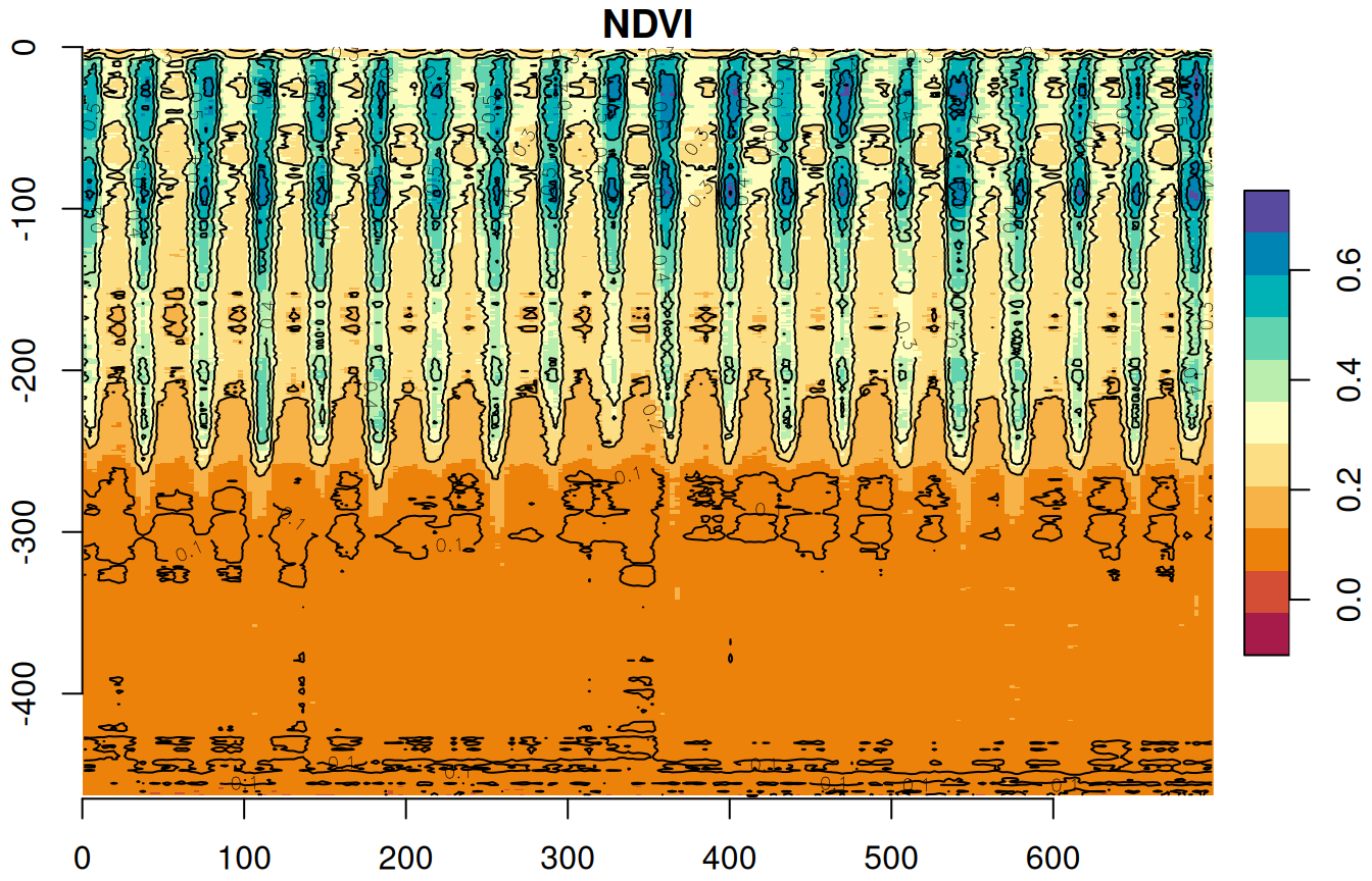

Figure 11.16: Row means of r over time

11.4 Processing trajectory data

11.4.1 The storms dataset

As another example of how list, split, and do.call can be useful when processing spatio-temporal data, we will transform a table of point locations over time to a line layer of trajectories. Our input data for this example is a data.frame object named storms (package dplyr):

library(dplyr)
storms = as.data.frame(storms)
vars = c('name', 'year', 'month', 'day', 'hour', 'long', 'lat')
storms = storms[, vars]

The storms table contains recorded storm locations at consecutive points over time:

head(storms)
##   name year month day hour  long  lat
## 1  Amy 1975     6  27    0 -79.0 27.5
## 2  Amy 1975     6  27    6 -79.0 28.5
## 3  Amy 1975     6  27   12 -79.0 29.5
## 4  Amy 1975     6  27   18 -79.0 30.5
## 5  Amy 1975     6  28    0 -78.8 31.5
## 6  Amy 1975     6  28    6 -78.7 32.4

For each storm record, we have the storm name (name), time (year, month, day, hour) and location (long, lat). The majority of storm records are given in consecutive 6-hour intervals (0, 6, 12, 18).

11.4.2 Setting storm IDs

To distinguish between individual storm tracks we need to have a unique ID variable. Our first pick could be to use storm name (name). However, storm name is not a good fit for an ID, because it is not unique. Many of the storm names are repeated for different storms in different years. For example, a storm named 'Josephine' appears in several different years between 1984 and 2008:

storms$year[storms$name == 'Josephine']
##   [1] 1984 1984 1984 1984 1984 1984 1984 1984 1984 1984 1984 1984 1984 1984 1984
##  [16] 1984 1984 1984 1984 1984 1984 1984 1984 1984 1984 1984 1984 1984 1984 1984
##  [31] 1984 1984 1984 1984 1984 1984 1984 1984 1984 1984 1984 1984 1984 1984 1984
##  [46] 1984 1984 1984 1984 1984 1984 1984 1984 1984 1984 1984 1990 1990 1990 1990
##  [61] 1990 1990 1990 1990 1990 1990 1990 1990 1990 1990 1990 1990 1990 1990 1990
##  [76] 1990 1990 1990 1990 1990 1990 1990 1990 1990 1990 1990 1990 1990 1990 1990
##  [91] 1990 1990 1990 1990 1990 1990 1990 1990 1990 1990 1990 1990 1990 1990 1990
## [106] 1990 1990 1990 1990 1990 1990 1990 1990 1990 1990 1990 1990 1990 1996 1996
## [121] 1996 1996 1996 1996 1996 1996 1996 1996 1996 1996 1996 1996 1996 1996 1996
## [136] 1996 1996 1996 1996 1996 1996 1996 1996 1996 1996 1996 1996 1996 1996 1996
## [151] 1996 1996 1996 1996 1996 1996 1996 1996 1996 1996 1996 1996 1996 1996 1996
## [166] 2002 2002 2002 2002 2002 2002 2002 2002 2002 2008 2008 2008 2008 2008 2008
## [181] 2008 2008 2008 2008 2008 2008 2008 2008 2008 2008 2008 2008 2008 2008 2008
## [196] 2008 2008 2008 2008 2008 2008 2008 2008 2008 2008 2008 2008 2020 2020 2020
## [211] 2020 2020 2020 2020 2020 2020 2020 2020 2020 2020 2020 2020 2020 2020 2020
## [226] 2020 2020 2020 2020 2020 2020

Consequently, we could choose to derive an ID that combines the storm name (name) and year (year), so that each name/year combination is unique. However, a storm can be spread over two different years, e.g., if it starts in December and ends in January of the following year! For example, one of the storms named 'Zeta' starts in December 30^th 2005 and ends in January 6^th 2006:

head(storms[storms$name == 'Zeta' & storms$year %in% 2005:2006, ])
##       name year month day hour  long  lat
## 10902 Zeta 2005    12  30    0 -35.6 23.9
## 10903 Zeta 2005    12  30    6 -36.1 24.2
## 10904 Zeta 2005    12  30   12 -36.6 24.7
## 10905 Zeta 2005    12  30   18 -37.0 25.2
## 10906 Zeta 2005    12  31    0 -37.3 25.6
## 10907 Zeta 2005    12  31    6 -37.6 25.7

tail(storms[storms$name == 'Zeta' & storms$year %in% 2005:2006, ])
##       name year month day hour  long  lat
## 10932 Zeta 2006     1   6   12 -49.6 23.1
## 10933 Zeta 2006     1   6   18 -50.2 23.3
## 10934 Zeta 2006     1   7    0 -51.4 23.7
## 10935 Zeta 2006     1   7    6 -52.7 24.2
## 10936 Zeta 2006     1   7   12 -54.2 24.8
## 10937 Zeta 2006     1   7   18 -55.7 26.3

Using a name/year combination as an ID will wrongly split the storm in two parts: 'Zeta 2005' and 'Zeta 2006'.

What we really need is a unique ID for each consecutive sequence of storm names, assuming that no two consecutive storms will be given the same name. This type of IDs can be automatically generated using function rleid (“Run Length Encoding ID”) from the data.table package. Assuming storms rows are in chronological order (otherwise we can sort them):

library(data.table)
storms$id = rleid(storms$name)

The storms table now has a new column named id, which contains a unique index for each storm:

head(storms)
##   name year month day hour  long  lat id
## 1  Amy 1975     6  27    0 -79.0 27.5  1
## 2  Amy 1975     6  27    6 -79.0 28.5  1
## 3  Amy 1975     6  27   12 -79.0 29.5  1
## 4  Amy 1975     6  27   18 -79.0 30.5  1
## 5  Amy 1975     6  28    0 -78.8 31.5  1
## 6  Amy 1975     6  28    6 -78.7 32.4  1

For example, using the id we can determine how many individual storms are there in the storms table (knowing that rleid produces IDs of consecutive numbers):

max(storms$id)
## [1] 638

11.4.3 To points

Our next step is to convert the storms table to a spatial point layer of the observed locations. The storms table can be converted to a point layer with st_as_sf, using the long and lat columns (Section 7.4):

library(sf)
pnt = st_as_sf(storms, coords = c('long', 'lat'), crs = 4326)

The resulting object pnt is an sf point layer with 19066 points:

pnt
## Simple feature collection with 19066 features and 6 fields
## Geometry type: POINT
## Dimension:     XY
## Bounding box:  xmin: -109.3 ymin: 7 xmax: 13.5 ymax: 70.7
## Geodetic CRS:  WGS 84
## First 10 features:
##    name year month day hour id           geometry
## 1   Amy 1975     6  27    0  1   POINT (-79 27.5)
## 2   Amy 1975     6  27    6  1   POINT (-79 28.5)
## 3   Amy 1975     6  27   12  1   POINT (-79 29.5)
## 4   Amy 1975     6  27   18  1   POINT (-79 30.5)
## 5   Amy 1975     6  28    0  1 POINT (-78.8 31.5)
## 6   Amy 1975     6  28    6  1 POINT (-78.7 32.4)
## 7   Amy 1975     6  28   12  1   POINT (-78 33.3)
## 8   Amy 1975     6  28   18  1     POINT (-77 34)
## 9   Amy 1975     6  29    0  1 POINT (-75.8 34.4)
## 10  Amy 1975     6  29    6  1   POINT (-74.8 34)

The point layer is shown in Figure 11.17:

plot(pnt)

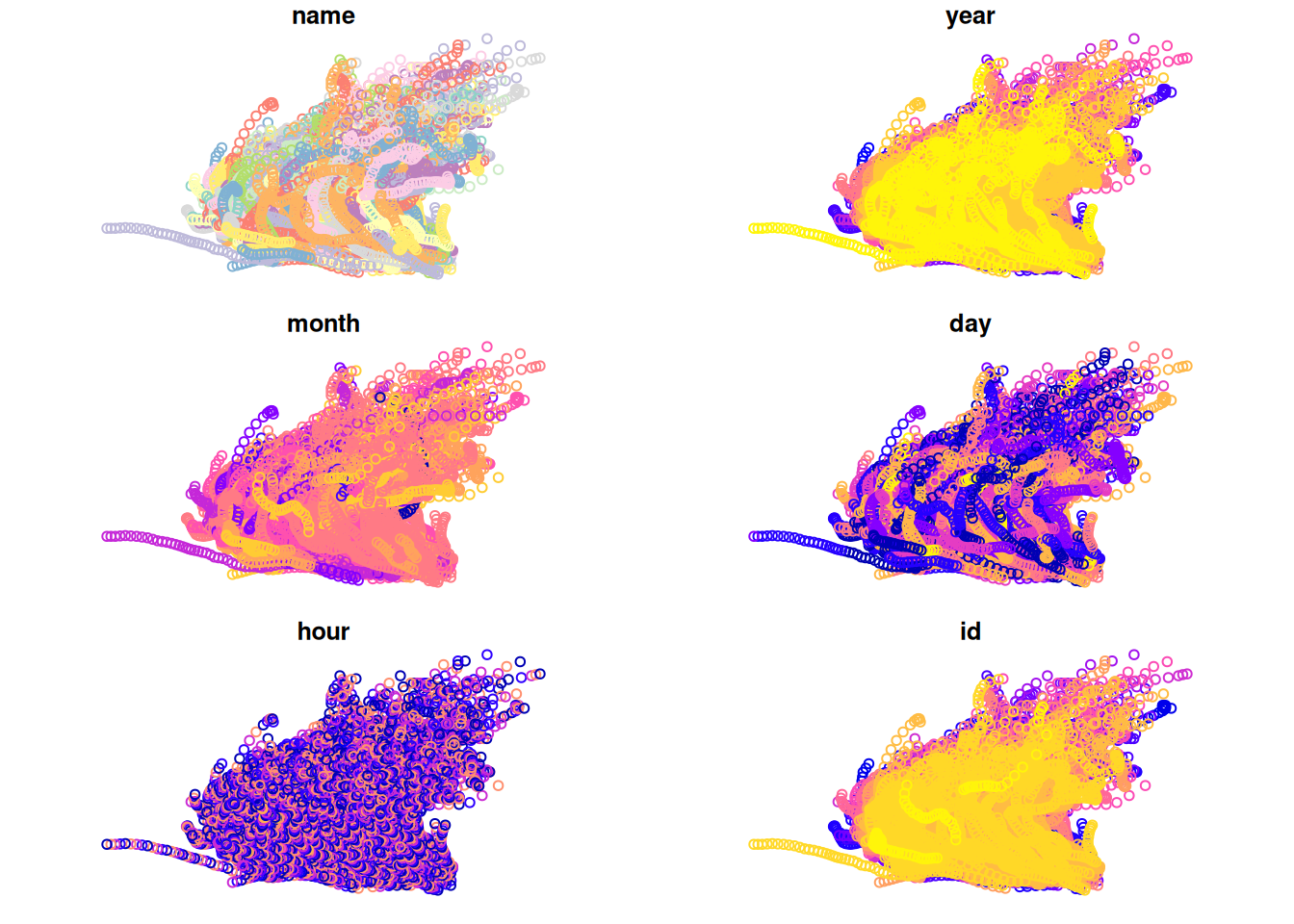
Figure 11.17: The storms points

11.4.4 Points to lines

To transform a point layer of object locations over time to a line layer of trajectories, we go through the following steps:

• Split the point layer to subsets of points for each storm
• Sort each group of points chronologically, earliest to latest
• Transform each of the point sequences to a line
• Combine the separate lines back to a single line layer

First, we split the point layer by storm ID (id), using the split function (Section 11.1.4). Remember that the sf class is a special case of a data.frame (Section 7.1.4), which is why split works with sf the same way as with a data.frame:

lines = split(pnt, pnt$id)

We now have a list of point sequences per storm. For example, the first list element contains 31 points for the first storm Amy in 1975:

lines[[1]]
## Simple feature collection with 31 features and 6 fields
## Geometry type: POINT
## Dimension:     XY
## Bounding box:  xmin: -79 ymin: 27.5 xmax: -48 ymax: 47
## Geodetic CRS:  WGS 84
## First 10 features:
##    name year month day hour id           geometry
## 1   Amy 1975     6  27    0  1   POINT (-79 27.5)
## 2   Amy 1975     6  27    6  1   POINT (-79 28.5)
## 3   Amy 1975     6  27   12  1   POINT (-79 29.5)
## 4   Amy 1975     6  27   18  1   POINT (-79 30.5)
## 5   Amy 1975     6  28    0  1 POINT (-78.8 31.5)
## 6   Amy 1975     6  28    6  1 POINT (-78.7 32.4)
## 7   Amy 1975     6  28   12  1   POINT (-78 33.3)
## 8   Amy 1975     6  28   18  1     POINT (-77 34)
## 9   Amy 1975     6  29    0  1 POINT (-75.8 34.4)
## 10  Amy 1975     6  29    6  1   POINT (-74.8 34)

Sorting the points, or making sure they are aready sorted, is essential to connect storm track points in chronological order. To sort the points we write a function that accepts a data.frame (or an sf) object and returns a sorted one based on the year, month, day and hour columns, in that order, using order (Section 4.6.2). The function is then applied on each storm, separately, using lapply (Section 11.1.3):

f = function(x) x[order(x$year, x$month, x$day, x$hour), ]
lines = lapply(lines, f)

Now each list element is a series of points in chronological order (or unchanged if it already was):

lines[[1]]
## Simple feature collection with 31 features and 6 fields
## Geometry type: POINT
## Dimension:     XY
## Bounding box:  xmin: -79 ymin: 27.5 xmax: -48 ymax: 47
## Geodetic CRS:  WGS 84
## First 10 features:
##    name year month day hour id           geometry
## 1   Amy 1975     6  27    0  1   POINT (-79 27.5)
## 2   Amy 1975     6  27    6  1   POINT (-79 28.5)
## 3   Amy 1975     6  27   12  1   POINT (-79 29.5)
## 4   Amy 1975     6  27   18  1   POINT (-79 30.5)
## 5   Amy 1975     6  28    0  1 POINT (-78.8 31.5)
## 6   Amy 1975     6  28    6  1 POINT (-78.7 32.4)
## 7   Amy 1975     6  28   12  1   POINT (-78 33.3)
## 8   Amy 1975     6  28   18  1     POINT (-77 34)
## 9   Amy 1975     6  29    0  1 POINT (-75.8 34.4)
## 10  Amy 1975     6  29    6  1   POINT (-74.8 34)

The first sequence is shown on Figure 11.18. We can see how the storm spans two different months and several different days (month and day panels).

plot(lines[[1]])

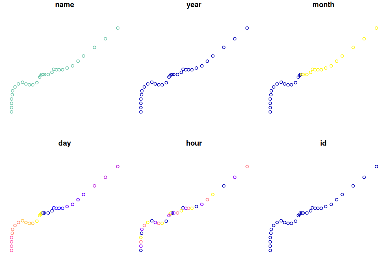
Figure 11.18: Points corresponding to the first storm in storms

11.4.5 Trajectory data

Our next step is to combine all POINT geometries to a single MULTIPOINT geometry. We use st_combine to do that (Section 8.3.4.3):

lines = lapply(lines, st_combine)

Each lines element is now a MULTIPOINT geometry (sfc):

lines[[1]]
## Geometry set for 1 feature 
## Geometry type: MULTIPOINT
## Dimension:     XY
## Bounding box:  xmin: -79 ymin: 27.5 xmax: -48 ymax: 47
## Geodetic CRS:  WGS 84
## MULTIPOINT ((-79 27.5), (-79 28.5), (-79 29.5),...

Why do you think all point attributes are lost as a result of applying st_combine?

The way the first list item looks when plotted is shown in Figure 11.19:

plot(lines[[1]])

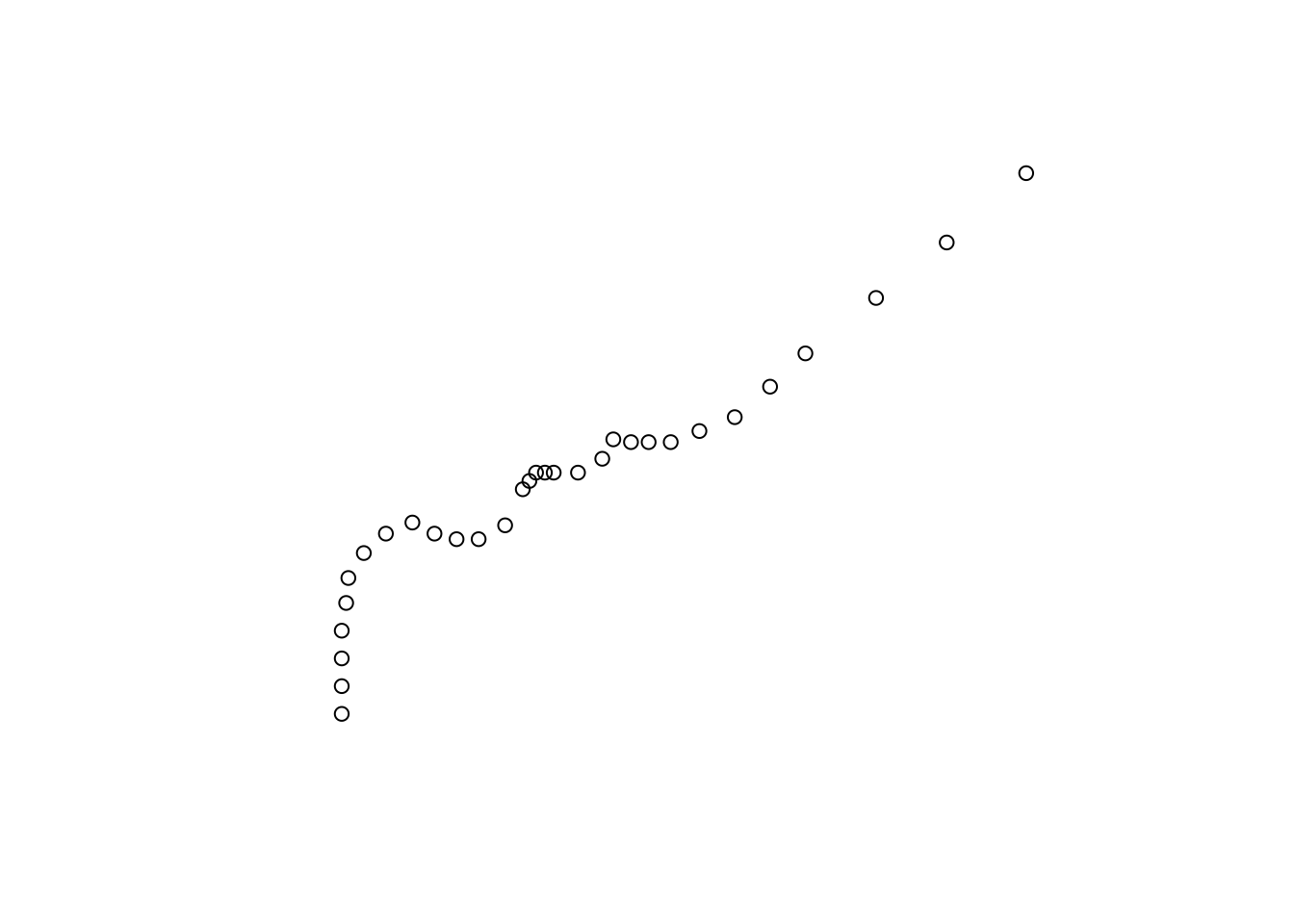
Figure 11.19: A point trajectory converted to MULTIPOINT

Next, each of the MULTIPOINT geometries can be cast (Section 8.3.4.4) to LINESTRING. Note that the additional fixed to parameter is passed from lapply to each of the st_cast function calls:

lines = lapply(lines, st_cast, to = 'LINESTRING')

Printing the first lines element reveals that the geometry type was indeed changed from MULTIPOINT to LINESTRING:

lines[[1]]
## Geometry set for 1 feature 
## Geometry type: LINESTRING
## Dimension:     XY
## Bounding box:  xmin: -79 ymin: 27.5 xmax: -48 ymax: 47
## Geodetic CRS:  WGS 84
## LINESTRING (-79 27.5, -79 28.5, -79 29.5, -79 3...

Accordingly, plotting shows a line instead of points (Figure 11.20):

plot(lines[[1]])

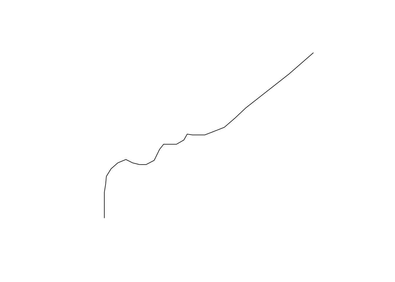
Figure 11.20: The LINESTRING created from MULTIPOINT

At this stage, we have a list of 638 individual LINESTRING geometries, one for each storm. The list can be combined back to an sfc geometry column with do.call (Section 11.1.5):

geom = do.call(c, lines)

Unlike in the previous example (Section 11.3.2) where we had a list of four elements (season_means), doing the above without do.call is not a viable option as we would have to type 638 arguments:

geom = c(
  lines[[1]],
  lines[[2]],
  ...,
  lines[[638]]
)

Here is the combined sfc:

geom
## Geometry set for 638 features 
## Geometry type: LINESTRING
## Dimension:     XY
## Bounding box:  xmin: -109.3 ymin: 7 xmax: 13.5 ymax: 70.7
## Geodetic CRS:  WGS 84
## First 5 geometries:
## LINESTRING (-79 27.5, -79 28.5, -79 29.5, -79 3...
## LINESTRING (-68.4 26, -69.5 26, -70.5 26.1, -71...
## LINESTRING (-69.8 22.4, -71.1 21.9, -72.5 21.6,...
## LINESTRING (-46.3 33.3, -47.5 33.6, -48.1 34.5,...
## LINESTRING (-55.2 17.6, -56.3 17.7, -57.3 17.8,...

We now have a geometry column geom, with one line per individual storm (Figure 11.21):

plot(geom)

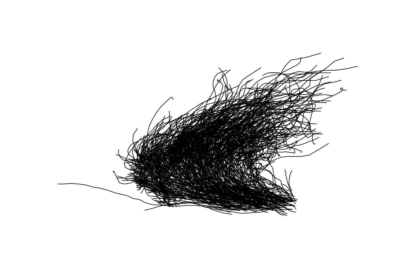
Figure 11.21: The LINESTRING geometries for all storms combined

What if we want to get back the other attributes of each storm, such as its name? To do that, we first need to attach storm IDs back to the geometries. We can rely on the fact that list names contain the original variable that was used for splitting the point layer, namely the storm IDs:

layer = st_sf(geom, data.frame(id = names(lines)))

The line layer is now an sf object with one attribute id:

layer
## Simple feature collection with 638 features and 1 field
## Geometry type: LINESTRING
## Dimension:     XY
## Bounding box:  xmin: -109.3 ymin: 7 xmax: 13.5 ymax: 70.7
## Geodetic CRS:  WGS 84
## First 10 features:
##    id                           geom
## 1   1 LINESTRING (-79 27.5, -79 2...
## 2   2 LINESTRING (-68.4 26, -69.5...
## 3   3 LINESTRING (-69.8 22.4, -71...
## 4   4 LINESTRING (-46.3 33.3, -47...
## 5   5 LINESTRING (-55.2 17.6, -56...
## 6   6 LINESTRING (-56.9 23, -57.2...
## 7   7 LINESTRING (-34.8 10.3, -35...
## 8   8 LINESTRING (-79.3 29.1, -79...
## 9   9 LINESTRING (-72.8 26, -73 2...
## 10 10 LINESTRING (-84 26, -82.7 2...

Plotting the layer shows the ID values per storm (Figure 11.22):

plot(layer)

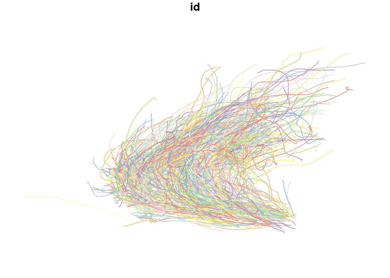
Figure 11.22: The storms line layer with storm ID

In case we need to, we can join other pieces of information from the original storms table back to layer, using aggregation (why?) followed by an ordinary join (Section 4.6) using the common column id.

11.4.6 Line length

Now that each storm is represented by a line, we can calculate spatial properties of the trajectories. For example, line length reflects the overall distance that each storm has traveled. The line lengths can be calculated using the st_length function (Section 8.3.2):

layer$length = st_length(layer)
layer
## Simple feature collection with 638 features and 2 fields
## Geometry type: LINESTRING
## Dimension:     XY
## Bounding box:  xmin: -109.3 ymin: 7 xmax: 13.5 ymax: 70.7
## Geodetic CRS:  WGS 84
## First 10 features:
##    id                           geom      length
## 1   1 LINESTRING (-79 27.5, -79 2... 3902720 [m]
## 2   2 LINESTRING (-68.4 26, -69.5... 3109017 [m]
## 3   3 LINESTRING (-69.8 22.4, -71... 3174193 [m]
## 4   4 LINESTRING (-46.3 33.3, -47... 1918095 [m]
## 5   5 LINESTRING (-55.2 17.6, -56... 5587288 [m]
## 6   6 LINESTRING (-56.9 23, -57.2... 4105575 [m]
## 7   7 LINESTRING (-34.8 10.3, -35... 8668566 [m]
## 8   8 LINESTRING (-79.3 29.1, -79... 1358420 [m]
## 9   9 LINESTRING (-72.8 26, -73 2... 2152455 [m]
## 10 10 LINESTRING (-84 26, -82.7 2... 1309996 [m]

Lengths can be transformed (see Section 8.3.2.2) to \(km\) units for convenience:

library(units)
layer$length = set_units(layer$length, 'km')
layer
## Simple feature collection with 638 features and 2 fields
## Geometry type: LINESTRING
## Dimension:     XY
## Bounding box:  xmin: -109.3 ymin: 7 xmax: 13.5 ymax: 70.7
## Geodetic CRS:  WGS 84
## First 10 features:
##    id                           geom        length
## 1   1 LINESTRING (-79 27.5, -79 2... 3902.720 [km]
## 2   2 LINESTRING (-68.4 26, -69.5... 3109.017 [km]
## 3   3 LINESTRING (-69.8 22.4, -71... 3174.193 [km]
## 4   4 LINESTRING (-46.3 33.3, -47... 1918.095 [km]
## 5   5 LINESTRING (-55.2 17.6, -56... 5587.288 [km]
## 6   6 LINESTRING (-56.9 23, -57.2... 4105.575 [km]
## 7   7 LINESTRING (-34.8 10.3, -35... 8668.566 [km]
## 8   8 LINESTRING (-79.3 29.1, -79... 1358.420 [km]
## 9   9 LINESTRING (-72.8 26, -73 2... 2152.455 [km]
## 10 10 LINESTRING (-84 26, -82.7 2... 1309.996 [km]

The result can also be visualized using mapview (Section 7.2.5) as follows:

library(mapview)
mapview(layer, zcol = 'length')

---