Chapter 3 Time series and function definitions
Last updated: 2025-02-06 09:27:38
Aims
Our aims in this chapter are:
- Learn to work with data which represent time (specifically, dates)
- Learn how to visualize our data, using graphical functions
- Learn to define custom functions
3.1 Dates and time series
3.1.1 Times and time series classes in R
Although our focus in this book is on spatial data, it is often necessary to work with times, and time series, when processing and analyzing spatial data. In particular, spatial data may contain temporal information—such as a time series of satellite images where each image is associated with a date (Figure 6.7), or a point layer representing a GPS recording where each point is associated with a time stamp. This type of data is known as spatio-temporal data. We will cover several specific methods to process spatio-temporal data in Chapter 11.
In R, there are several special classes for representing times and time-series (time+data). First of all, let us define what do we mean by those terms:
- The term times refers to a series of values that represent specific points in time, at a given resolution, typically either:
- days—e.g.,
2021-10-26), or - (sub-)seconds—e.g.,
2021-10-26 15:21:37.
- days—e.g.,
- The term time series refers to the combination of times and corresponding values, or measurements, associated with those times. A time series may be:
- univariate, when the times are associated with one series (e.g., a time series of daily rainfall), or
- multivariate, when the times are associated with more than one series of values representing different variables (e.g., a time series of daily rainfall, minimum temperature, maximum temperature, and average humidity).
Here is a list of commonly used classes to represent times, and time series, in R:
- Times:
Date—To represent times at daily resolution (Section 3.1.2)POSIXctandPOSIXlt—To represent times at second (or sub-second) resolution
- Time series:
tszoo(packagezoo)xts(packagexts)
In this book, we will only be working with the Date class, which is used to represent times of type date.
3.1.2 Working with Date objects
3.1.2.1 Today’s date
The simplest data structure for representing times is Date, used to represent dates (without time of day). For example, we can get the current date with Sys.Date:
The printed output has the same appearance as that of character vectors. Calling the class function (Section 1.3.11) on x, however, reveals this is indeed an object of the specialized class Date:
3.1.2.2 Converting character to Date
We can also convert character values to Date, using as.Date. That way, we can create a Date object representing not just today’s date, but any date we want:
When the character values are in the standard date format known as ISO 8601 (YYYY-MM-DD), such as in the above example, the as.Date function works without any additional arguments. However, when the character values are in a non-standard format, we need to specify the format definition with format, using date component symbols.
Table 3.1 lists the most commonly used symbols for specifying date formats in R11. The date format specification basically tells as.Date which formats are being used to convey the year/month/day information, in what order, and whether there are additional fixed characters (such as - or /). For example, using the Date format symbols, the standard format is specified as "%Y-%m-%d".
| Symbol | Example | Meaning |
|---|---|---|
%d |
"15" |
Day |
%m |
"08" |
Month, numeric |
%b |
"Aug" |
Month, 3-letter |
%B |
"August" |
Month, full |
%y |
14 |
Year, 2-digit |
%Y |
2014 |
Year, 4-digit |
Before going into examples of date formatting, it is useful to set the standard "C" locale in R. That way, we make sure that month names (%B and %b) are interpreted in English. Setting the standard "C" local is done with the following expression:
For example, converting the following character date—which is in a non-standard format—to Date fails when format is not specified:
as.Date("07/Aug/12")
## Error in charToDate(x): character string is not in a standard unambiguous format
Specifying the right format, which is "%d/%b/%y" in this case, leads to a successful conversion:
What will be the result if we used
format="%y/%b/%d"(switching%dand%y) in the above expression?
Here is another example with a different non-standart format ("%Y-%B-%d"):
3.1.2.3 Converting Date to character
The opposite conversion, from Date to character, is done using function format:
Remember that Date and character objects are printed exactly the same way! We have to use class to figure out which class we are dealing with.
The format function, by default, returns a text string with all three date components in the standard YYYY-MM-DD (or "%Y-%m-%d") format. Using the format argument and the same notation as in as.Date (Table 3.1), however, we can compose different date formats, or extract individual date components out of a Date object:
Note that format consistently returns a character, even when the result contains nothing but numbers, as in "%d" or "%Y". When necessary, we can convert from character to numeric using the as.numeric function:
3.1.2.4 Arithmetic operations with dates
At this point, you may ask yourself why do we even bother to create Date objects, dealing with date formats, instead of simply working with character dates. The reason is that representing dates as Date makes it possible to do extremely useful operations, such as date arithmetic.
Date arithmetic means that Date objects act like numeric vectors, with respect to certain operations that make sense for dates, such as:
- Conditional operators—Comparing which date is earlier or later
- Subtraction between two dates—Calculating the time difference between two dates
- Addition or subtraction between a date and a number—Calculating the date X days from the given date
- Creating sequences with
seq—Creating date sequences
We will now see an example of each operation. Starting with conditional operators, the following expression uses a conditional operator to check whether today’s date is after 2013-01-01:
The subtraction operator (-) can be used to calculate the time difference between two dates:
The result is an object of class difftime:
which can be converted to number(s), using as.numeric, along with the unit we are interested in:
A date, plus or minus a number, gives a new date, the specified days before or after the given one. For example:
Finally, using the seq function—which we are already familiar with (Section 2.3.6.2)—we can create a sequence of consecutive dates. For example, the following expression creates a sequence of dates:
- starting at
"2018-10-14", - ending at (or before)
"2019-01-11", and - with a step size of 7 days
seq(from = as.Date("2018-10-14"), to = as.Date("2019-01-11"), by = 7)
##  [1] "2018-10-14" "2018-10-21" "2018-10-28" "2018-11-04" "2018-11-11"
##  [6] "2018-11-18" "2018-11-25" "2018-12-02" "2018-12-09" "2018-12-16"
## [11] "2018-12-23" "2018-12-30" "2019-01-06"
As you can see, Date is a vector-like class. Most of the methods we learned about vectors, such as subsetting or recycling, apply to Date objects exactly the same way as to numeric, character, and logical vectors.
3.1.3 Time series
In this book, we will not be working with specialized time series classes, such as ts (Section 3.1.1). Instead, we will use the straightforward “manual” approach of treating a sequence of measurements and a corresponding sequence of times, referring to when those measurements were taken, as a time series. For straightforward operations, such as subsetting or calculating time differences, this approach has the advantage that we do not need to learn about any special classes other than vectors. However, for using specialized time-series calculations, such as focal filtering or filling of missing values (which is beyond the scope of this book), we do need to use specialized classes such as zoo and xts (Section 3.1.1).
For example, let’s define two vectors:
- Water level in Lake Kinneret—a
numericvector namedvalue - The corresponding date when water level was measured—a
Datevector namedtime
The water measurements were taken in May and in November, in each year during 1991-2011.
The values of value are specified “manually”:
value = c(-211.92, -212.79, -208.8, -209.52, -208.84, -209.72, -209.12,
-210.94, -209.01, -210.85, -209.60, -211.40, -210.24, -212.01,
-210.46, -212.25, -211.76, -213.00, -211.92, -213.71, -213.13, -214.78,
-213.18, -214.34, -209.74, -210.93, -208.92, -210.69, -209.73,
-211.64, -210.68, -212.03, -211.1, -212.60, -212.18, -214.23,
-213.26, -214.33, -212.65, -213.89, -212.37, -213.68)
The values of time are constructed using rep, paste0, and as.Date:
time = rep(1991:2011, each = 2)
time = paste0(time, c("-05-15", "-11-15"))
time = as.Date(time)
time
##  [1] "1991-05-15" "1991-11-15" "1992-05-15" "1992-11-15" "1993-05-15"
##  [6] "1993-11-15" "1994-05-15" "1994-11-15" "1995-05-15" "1995-11-15"
## [11] "1996-05-15" "1996-11-15" "1997-05-15" "1997-11-15" "1998-05-15"
## [16] "1998-11-15" "1999-05-15" "1999-11-15" "2000-05-15" "2000-11-15"
## [21] "2001-05-15" "2001-11-15" "2002-05-15" "2002-11-15" "2003-05-15"
## [26] "2003-11-15" "2004-05-15" "2004-11-15" "2005-05-15" "2005-11-15"
## [31] "2006-05-15" "2006-11-15" "2007-05-15" "2007-11-15" "2008-05-15"
## [36] "2008-11-15" "2009-05-15" "2009-11-15" "2010-05-15" "2010-11-15"
## [41] "2011-05-15" "2011-11-15"
These two vectors, taken together, comprise a univariate time series, where:
timespecifies the time of measurementvaluespecifies the values of the measured variable, namely the water level of lake Kinneret
It should be noted, at this point, that a table is more natural for representing a collection of corresponding vectors, such as the times and measurements that comprise a time series, as shown below. A table in R is represented with a class called data.frame, which we learn about in Chapter 4. For now, here is what the first six rows of the data.frame containing the same data would look like:
3.1.4 Operations with time series
Let’s move on to demonstrate common questions we can ask about a time series, how they can be answered in R. We will use several methods we already learned earlier (Chapter 2), and a new one (Section 3.1.5).
What was the average water level in Lake Kinneret, based on all measurements combined?
Did the water level ever go below -213.2 (the “lower red line”)? We can find out using the any function (Section 2.4.1)12:
Was the water below
-214.4(the “black line”, where irreversible damage occurs)? If so, how many measurements below the black line were made?
How can we find out the dates when the measured water level was below -213.2? We can use the logical vector value < -213.2 to subset (Section 2.3.10.2) the time vector:
time[value < -213.2]
## [1] "2000-11-15" "2001-11-15" "2002-11-15" "2008-11-15" "2009-05-15"
## [6] "2009-11-15" "2010-11-15" "2011-11-15"
How can we find out the years and months when the water level was below -213.2? We can first “extract” those components out of the Date:
Then, subset those vectors:
3.1.5 Consecutive differences
The diff function can be used to create a vector of differences between consecutive elements. For example, suppose we have the vector:
diff(x) returns a vector with the values c(8-15, 23-8, 24-23):
Note that the length of diff(x) is one element less than x, because we don’t have the difference for the first, or last, element, depending how you look at it. To keep x and diff(x) aligned, we can add an NA at the beginning (or end) of the vector. For example, an NA at the beginning implies that the difference between the first element and the previous one is not available:
Here is an example of applying the same expression on value, to calculate the change in Kinneret water level between consecutive measurements separated by 6 months:
d_value = c(NA, diff(value))
d_value
##  [1]    NA -0.87  3.99 -0.72  0.68 -0.88  0.60 -1.82  1.93 -1.84  1.25 -1.80
## [13]  1.16 -1.77  1.55 -1.79  0.49 -1.24  1.08 -1.79  0.58 -1.65  1.60 -1.16
## [25]  4.60 -1.19  2.01 -1.77  0.96 -1.91  0.96 -1.35  0.93 -1.50  0.42 -2.05
## [37]  0.97 -1.07  1.68 -1.24  1.52 -1.31
Now we can find out, for example, which time period had the biggest water level decrease or increase in water level13, using which.min and which.max (Section 2.4.3), respectively:
time[which.min(d_value)]  ## Date of biggest decrease
## [1] "2008-11-15"
time[which.max(d_value)]  ## Date of biggest increase
## [1] "2003-05-15"
Recall that which.min and which.max ignore NA values (Section 2.4.3), which is appropriate in this case.
3.2 Graphics
3.2.1 The plot function
The function named plot is the basic graphical function in R. plot is also an example of a generic function. Generic functions are functions that do different things when we pass different classes as their input, according to the predefined method for that class. For example, plot displays different graphical output depending on the type of input(s). Given a numeric vector, plot displays its values in a two dimensional plot. Given a raster or a vector layer, plot displays the layer in the form of a map, as we will see later on (Sections 5.3.7 and 7.8, respectively).
Here is an example of plotting a numeric vector with plot (Figure 3.1):
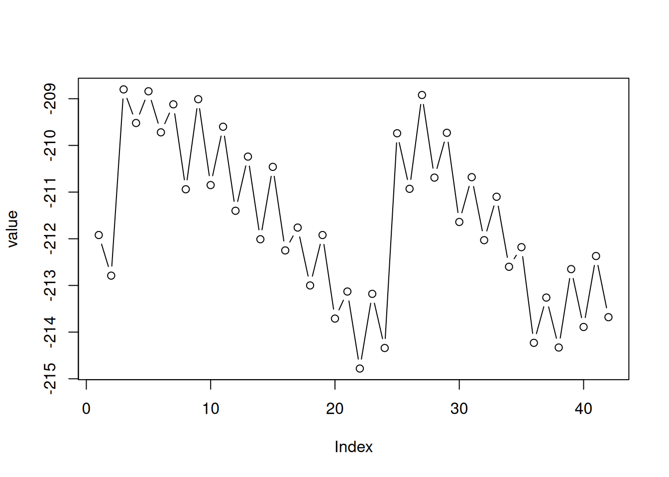
Figure 3.1: Plot of the value vector
Note that:
- Vector indices are displayed on the x-axis
- Vector values are displayed on the y-axis
The type="b" argument means draw both points and lines. Other useful options for type include:
type="p"for points (the default)type="l"for linestype="o"for overplotted lines and points
When working with RStudio, the graphical output should appear in a separate panel (Figure 1.9). Graphical output can also be “diverted” to a file, using format-specific functions such as pdf, jpeg, png, svg, etc. Check out the Examples section in the documentation of those functions to see how they can be used.
Try executing the above plot expression with all possible
typearguments, to see what the results look like.
3.2.2 Specifying x-axis values
If we pass two vectors to plot, the values of the first vector appears on the x-axis, while the values of the second vector appear on the y-axis. For example, we can put the times of water level measurement on the x-axis, as follows (Figure 3.2). The plot function automatically places labels (such as years) when the x-axis values are a Date vector.
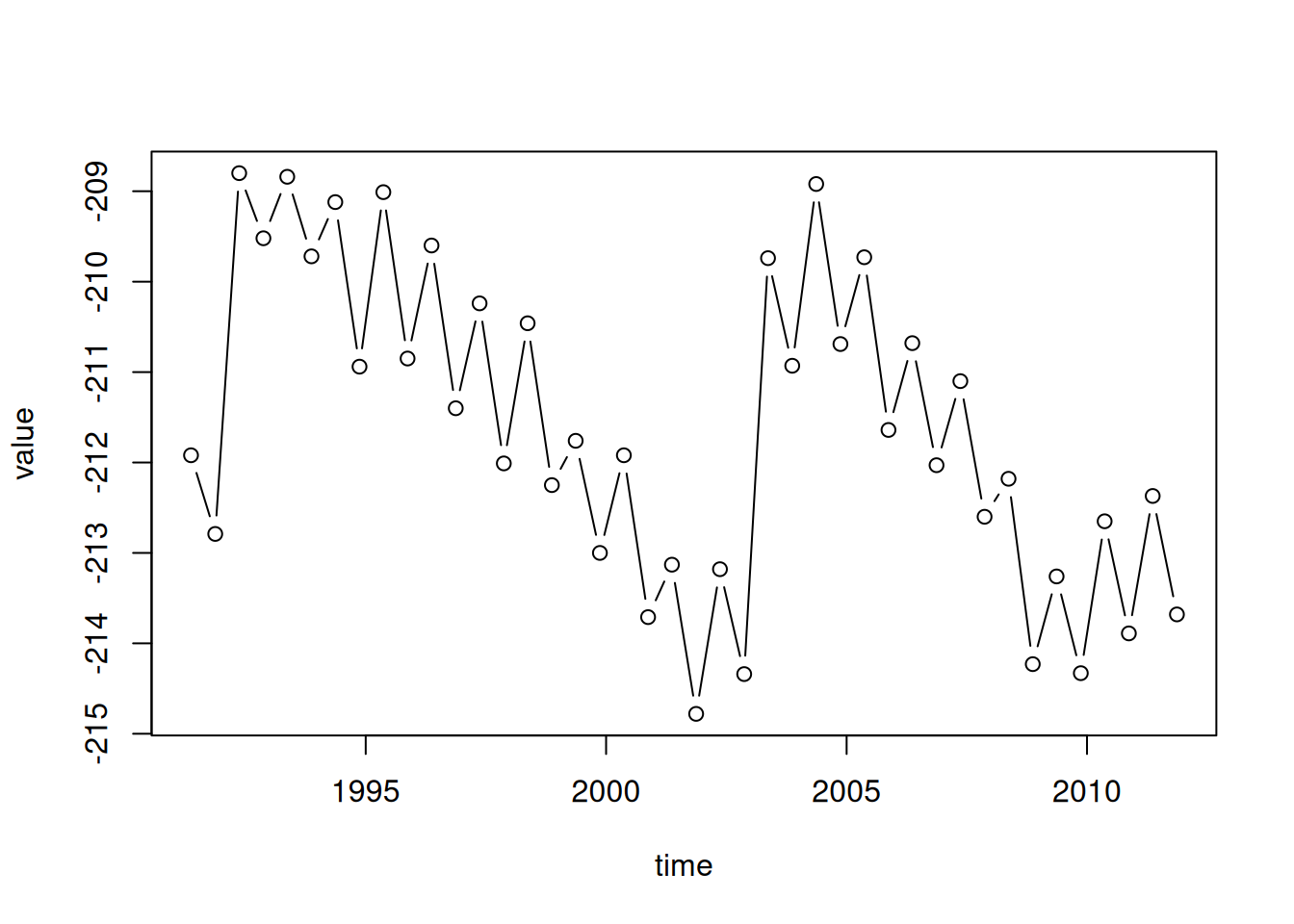
Figure 3.2: value as function of time
3.2.3 Horizontal lines
We can add a horizontal line displaying the Kinneret “red line” and “black line” using abline with the h parameter. The h parameter determines the y-axis value for the horizontal line. Note that abline draws an additional “layer” in an existing graphical device, which was initiated with plot (Figure 3.3). We are also using:
col—to specify a different line color (such as"red")lty—to specify line type (such as"dashed")
plot(time, value, type = "b")
abline(h = -213.2, col = "red", lty = "dashed")
abline(h = -214.4, lty = "dashed")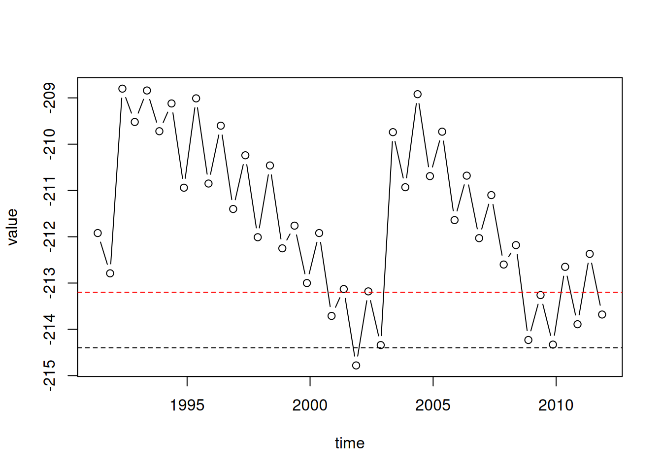
Figure 3.3: Adding a horizontal line with abline
3.2.4 Plotting multiple series
Additional “layers”, such as other series of measurements, can be added to an existing plot using the functions points and lines. For example, the following code section draws the May and November measurements as separate time series in the same plot. Again, we are using the graphical parameter col to specify a different line color. In addition, we are setting the y-axis range with ylim to make sure both time series fit inside the displayed range. The ylim argument needs to be a vector of length two, the minimum and the maximum (Figure 3.4):
plot(
  time[month == 5],
  value[month == 5],
  ylim = range(value),
  type = "b",
  col = "darkred"
)
lines(
  time[month == 11],
  value[month == 11],
  type = "b",
  col = "darkblue"
)
abline(h = -213.2, col = "red", lty = "dashed")
abline(h = -214.4, lty = "dashed")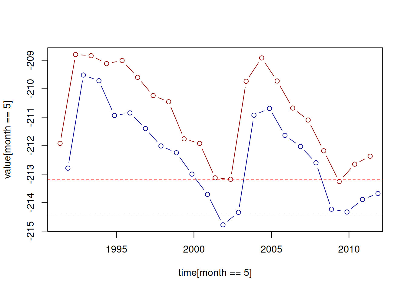
Figure 3.4: Adding a second series with lines
3.2.5 Axis labels
One more important plot detail is the axis labels. Axis labels can be set using the xlab and ylab parameters of plot, as follows (Figure 3.5):
plot(time, value, type = "b", xlab = "Time", ylab = "Elevation (m)")
abline(h = -213.2, col = "red", lty = "dashed")
abline(h = -214.4, lty = "dashed")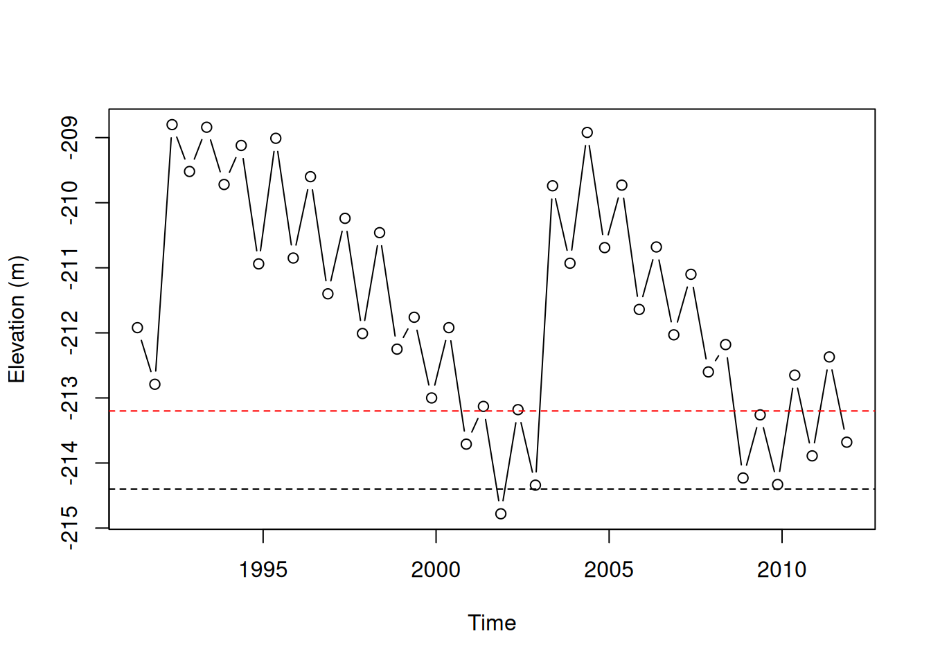
Figure 3.5: Setting axis labels
3.2.6 Text annotations
Finally, we can add text annotations on top of an existing plot, using the text function. The text function requires:
x—A numeric (orDate) vector of x-axis positionsy—A vector of y-axis positionslabels—A vector of text labels
Given these inputs, text adds the text values (labels) in the specified x/y locations (x,y). Another useful parameters of text is pos:
pos—Position where the label will be placed relatively to the x/y location, with possible values:NULL(default)—exactly atc(x,y)1—below2—left3—above4—right
Here is an example of using text to annotate the time series, marking the times of maximum increase and maximum decrease in water levels, and the associated change in water level (Figure 3.6). These expressions are quite complex, but they are mostly composed of vector operations we learned earlier. The one thing that is new here is the use of round(x,2), to round the number x to two decimal places.
plot(time, value, xlab = "Time", ylab = "Elevation (m)", type = "b")
text(
  time[which.max(d_value)],
  value[which.max(d_value)],
  paste0("+", round(d_value[which.max(d_value)], 2)),
  pos = 3,
  col = "blue"
)
text(
  time[which.min(d_value)],
  value[which.min(d_value)],
  round(d_value[which.min(d_value)], 2),
  pos = 3,
  col = "red"
)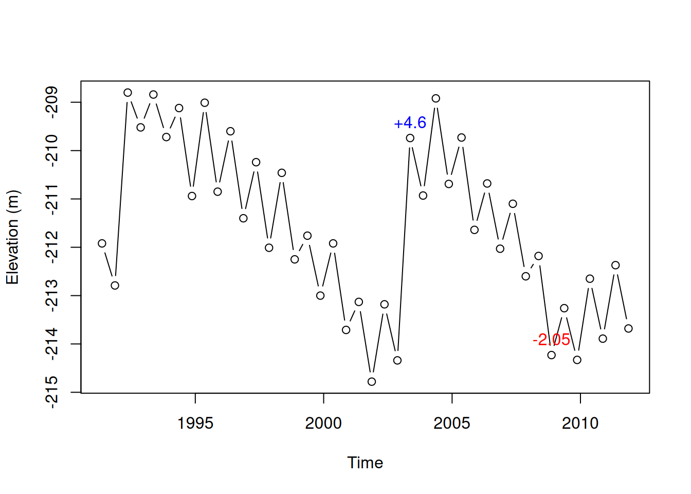
Figure 3.6: Times of biggest increase (2003) and decrease (2008) in the Kinneret water level time series
3.3 Defining custom functions
3.3.1 Function definition components
In Section 1.3.6, we learned that a function call is an instruction to execute a particular function, as in:
The function itself is actually an object containing code, which is loaded into the RAM, and can be executed with specific arguments. So far, we met functions defined in the default R packages (e.g., mean, seq, length, etc.). Later on we will also use functions from external packages 5.3.3. In this section, we learn how to define our own custom functions.
Here is an example of a function definition, where we define a function named add_five that has one parameter x. The function calculates and returns the sum of x and 5:
Let us go over the components of a function definition expression in R. The function definition expression is composed of:
- A function name (
add_five) - The assignment operator (
=) - The
functionkeyword (function) - Parameter(s), inside parentheses and separated by commas (
(x)) - Curly brackets (
{) - Code (
x_plus_five = x + 5) - Returned value (
return(x_plus_five)) - Curly brackets (
})
3.3.2 Function definition vs. function call
The idea is that the code inside the function gets executed each time the function is called. For example, the function we just defined, add_five, can be used to calculate the sum of various numbers and five. Here is, again, the add_five function definition:
And here are two function calls of the add_five function, using different arguments 5 and 77:
Note the returned values, 10 and 82, printed in the console.
3.3.3 Local variables
When we make a function call, the values we pass as function arguments are assigned to local variables which the function code can use. Those local variables are not accessible in the global environment. For example, even though we just executed two function calls of add_five, where the local variable x_plus_five was defined, x_plus_five is not available in the global environment:
3.3.4 Returned value
Every function returns a value. We can assign the returned value to a variable, in case we want to keep it in memory for later use:
A return expression, such as the one we used in add_five:
is optional, and can be omitted.
If the return expression is omitted, the returned value is the result of the last expression in the function body. The following alternative definition of add_five, where the assignment and the return expressions were omitted, is therefore identical:
We can also omit the { and } parentheses in case the code consists of a single expression. Therefore the add_five function definition can be simplified to this:
3.3.5 Default arguments
Default arguments (Section 2.3.7) can be specified as part of the function definition. In case there is a default value, we can skip that parameter in function calls.
For example, the following definition of add_five does not specify a default value for x. Therefore, trying to call add_five without passing an argument for x gives an error:
add_five = function(x) x + 5
add_five()
## Error in add_five(): argument "x" is missing, with no default
The following, an alternative definition, does specify the default value of 0 for x. The default value is then used when calling the function without specifying x:
3.3.6 Argument types
There are no restrictions for the classes and dimensions of arguments a function can accept, as long as we did not set such restrictions ourselves, e.g., using conditionals (Section 4.2.2). However, we get an error if one of the expressions in the function code is illegal given the arguments.
For example, even though we may have intended add_five to be used with vectors of length 1, it also works for vectors of length >1, adding five to each element, because 5 in x+5 is recycled (Section 2.3.5):
However, passing a character value gives an error, because the internal expression x+5 cannot be executed when x is not numeric (Section 1.3.7):
3.3.7 More examples
As another example, let’s define a function named last_minus_first which accepts a vector and returns the difference between the last and the first elements:
Here are two function calls to demontrate that our function indeed works as expected:
Define a function named
modifythat accepts three arguments:
xindexvalueThe function assigns
valueinto the element at theindexposition of vectorx. The function returns the modified vectorx, as shown below.
The full list of date format symbols can be found in
?strptime↩︎When typing
value < -213, make sure there is a space between<and-. Otherwise the combination is interpreted as an assignment operator<-!↩︎Note that, when comparing rates of change, which is what we inmlicitly do with
which.min(d_value)andwhich.max(d_value), we need to divide the differences (diff(value)) by the time differences (diff(time)). In this particular dataset, this does not matter, because the time differences between measurements are fixed at ~6 months.↩︎