G Exercise 05
Last updated: 2025-02-06 09:33:53
G.2 Question 1
- Recreate the DEM of the Carmel area in UTM, as shown in the right panel in Figure 9.10, using the following code section:
library(stars)
dem1 = read_stars('data/srtm_43_06.tif')
dem2 = read_stars('data/srtm_44_06.tif')
pol = st_read('data/israel_borders.shp', quiet = TRUE)
dem = st_mosaic(dem1, dem2)
dem = dem[, 5687:6287, 2348:2948]
names(dem) = 'elevation'
dem = st_warp(src = dem, crs = 32636, method = 'near', cellsize = 90)- Calculate a point geometry of the peak of the Carmel mountain, by finding the centroid of the pixel that has the highest elevation in the image.
- Calculate the nearest point in the Mediterranean sea from the peak, assuming the sea area is all of the
NApixels in the image. (Hint: calculate the distances from the peak to allNApixels, converted to points, then usewhich.minto find the nearest one.) - Plot the DEM, the peak, the nearest “sea” point, the line connecting them, and the distance, as shown in Figure G.1.
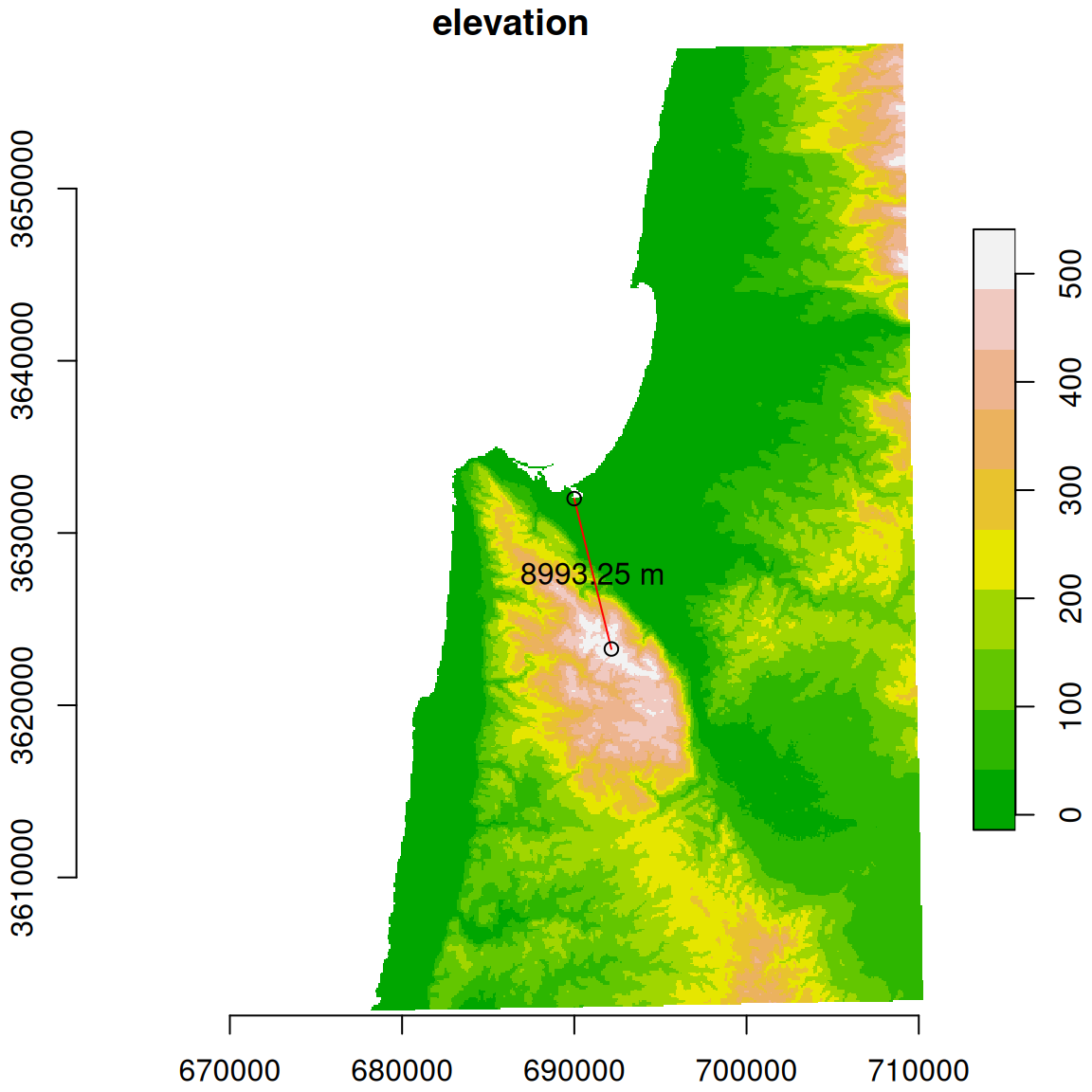
Figure G.1: Length of the shortest line between Carmel mountain peak and the Mediterranean sea
(50 points)
G.3 Question 2
- Read the
MOD13A3_2000_2019.tifraster, with monthly NDVI values, into astarsobject namedr, then reproject it to UTM withst_warp(r, crs = 32636).
- Use
dates.csvto assign date values to raster bands (see Section 6.3.2). - Read the Shapefile named
nafot.shp, which includes polygons of “Nafa” administrative regions in Israel, and reproject it to UTM as well. - Calculate the average NDVI for each polygon in each date.
- Plot the resulting time series of average NDVI for each of the “Nafot”, as shown in Figure G.2. Hint: you can start from an empty plot using
plot(..., col=NA), then add the NDVI times series usinglinesinforloop; see Section 6.1.3. - The time series of “Nafa” where the highest and lowest average NDVI were observed, during the studied period, need to be highlighted in blue and red, respectively. The other “Nafa” should be displayed in grey. Don’t specific use “Nafa” indices (such as
6) or names (such as'Golan'), instead calculate the required indices in your code.
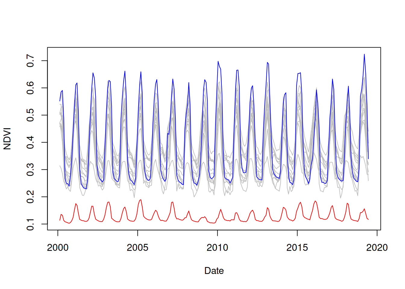
Figure G.2: Average NDVI over time in “Nafa” polygons, “Nafa” with highest and lowest observed average NDVI are marked in blue and red, respectively
(50 points)