Chapter 8 Geometric operations with vector layers

Last updated: 2024-07-28 11:43:46

Aims

Our aims in this chapter are:

Learn how to join data to a vector layer, by attributes or by location
Learn to make geometric calculations with vector layers

We will use the following R packages:

sf
units

8.1 Spatial join

For most of the examples in this chapter, we are going to use the US counties and three airports layers (Section 7.7):

library(sf)
airports = st_read('data/airports.geojson', quiet = TRUE)
county = st_read('data/USA_2_GADM_fips.shp', quiet = TRUE)

transformed to the US National Atlas projection (Section 7.9.2):

airports = st_transform(airports, 9311)
county = st_transform(county, 9311)

Join by spatial location, or spatial join, is one of the most common operations in spatial analysis. In a spatial join we are “attaching” attributes from one layer to another, based on their spatial relations. In ArcGIS this is done using “Join data from another layer based on spatial location” (Figures 8.1–8.2).

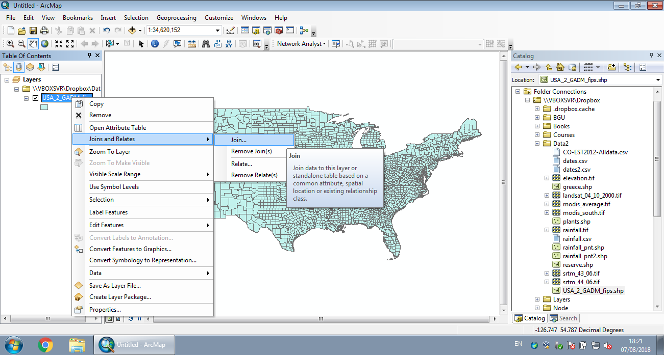
Figure 8.1: Join by location in ArcGIS (Step 1)

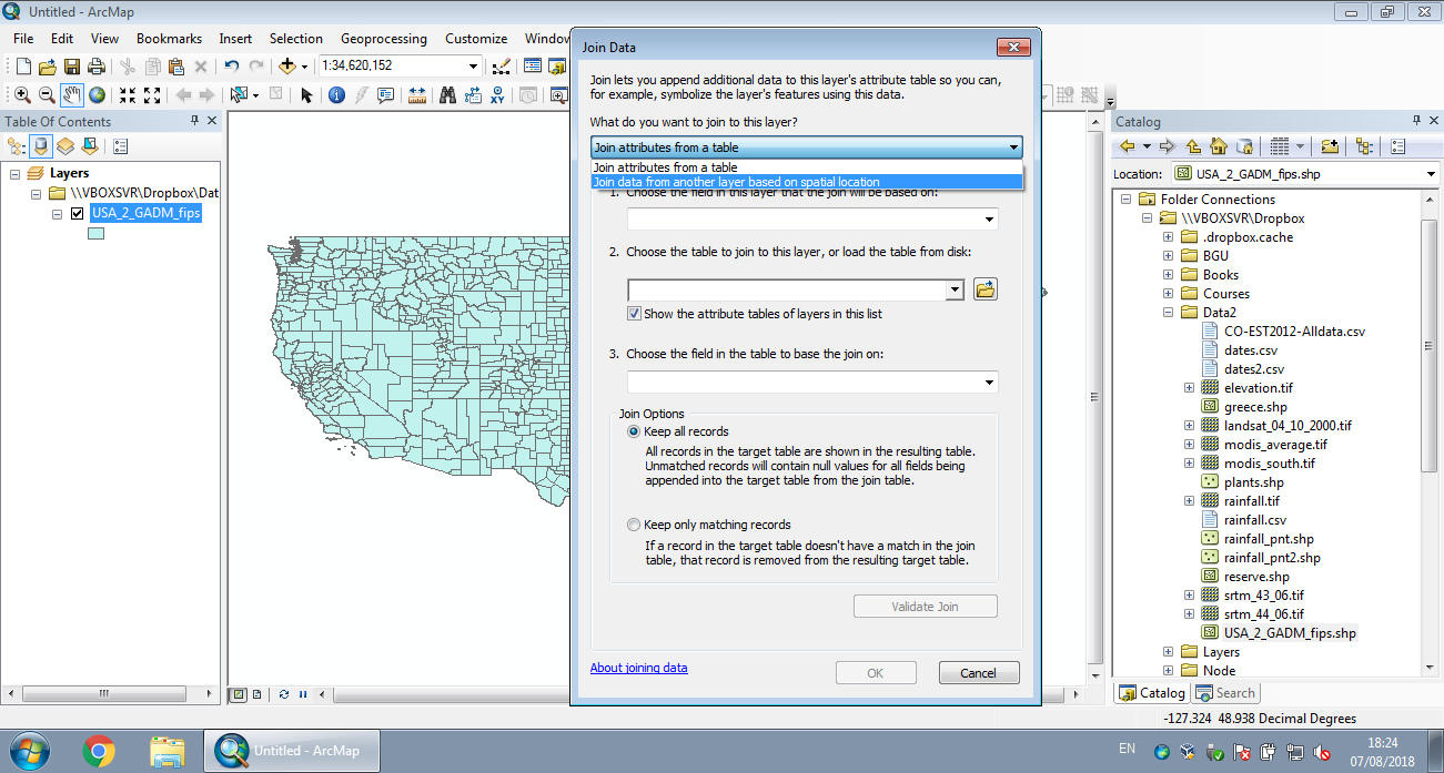
Figure 8.2: Join by location in ArcGIS (Step 2)

To simplify our demonstration of spatial join between the airports and counties layers, we will create a subset of the counties of New Mexico only, since all three airports are located in that state:

nm = county[county$NAME_1 == 'New Mexico', ]

Figure 8.3 shows the geometry of the nm and airports layers. Note that the pch parameter determines point shape (see ?points), while cex determines point size (Section 7.8):

plot(st_geometry(nm))
plot(st_geometry(airports), col = 'red', pch = 16, cex = 2, add = TRUE)

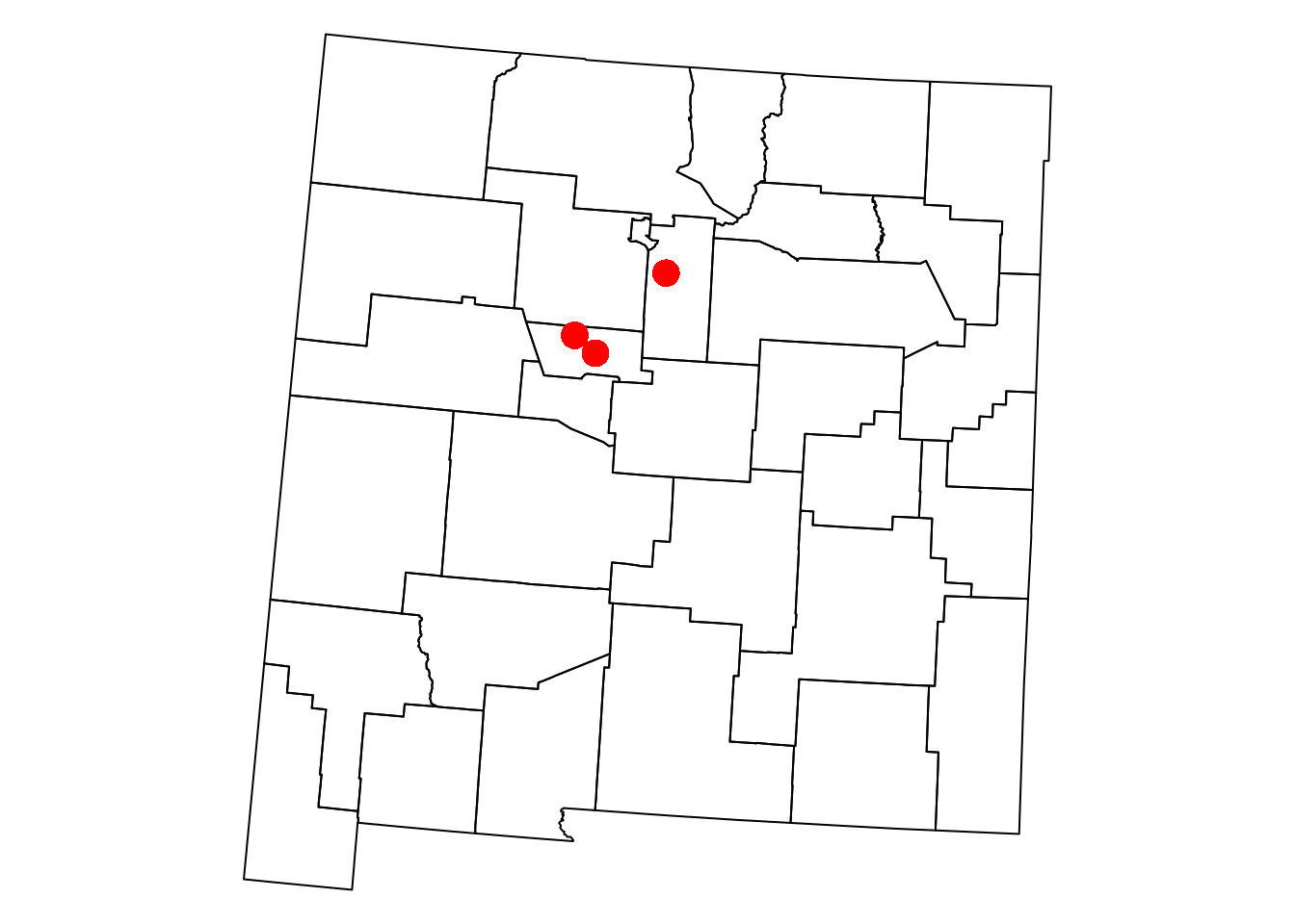
Figure 8.3: The nm and airports layers

Given two layers x and y, a function call of the form st_join(x,y) returns the x layer along with matching attributes from y. The default join type is by intersection, meaning that two geometries are considered matching if they intersect. Other join types can be specified using the join parameter (see ?st_join).

For example, the following expression joins the airports layer with the matching nm attributes. The resulting layer contains all three airports with their original geometry and name attribute, plus the NAME_1, NAME_2, TYPE_2, and FIPS of the nm feature that each airport intersects with:

st_join(airports, nm)
## Simple feature collection with 3 features and 5 fields
## Geometry type: POINT
## Dimension:     XY
## Bounding box:  xmin: -620409.7 ymin: -1080157 xmax: -552795.4 ymax: -1021040
## Projected CRS: NAD27 / US National Atlas Equal Area
##                        name     NAME_1     NAME_2 TYPE_2  FIPS
## 1 Albuquerque International New Mexico Bernalillo County 35001
## 2           Double Eagle II New Mexico Bernalillo County 35001
## 3        Santa Fe Municipal New Mexico   Santa Fe County 35049
##                     geometry
## 1 POINT (-605057.1 -1080157)
## 2 POINT (-620409.7 -1067009)
## 3 POINT (-552795.4 -1021040)

What do you think will happen if we reverse the order of the arguments, as in st_join(nm,airports)? How many features is the result going to have, and why?

8.2 Spatial subsetting

In Section 7.6 we learned how to subset sf vector layers based on their attributes, just like an ordinary data.frame (Section 4.1.5). We can also subset an sf layer based on its intersection with another layer. Spatial subsetting, or subsetting by location, uses the same [ operator, using the other layer as the “index”. Namely, an expression of the form x[y,]—where x and y are vector layers—returns a subset of x features that intersect with y.

For example, the following expression creates a new layer nm1, with only those nm counties that intersect with the airports layer:

nm1 = nm[airports, ]

The subset is shown in light blue in Figure 8.4:

plot(st_geometry(nm))
plot(st_geometry(nm1), col = 'lightblue', add = TRUE)
plot(st_geometry(airports), col = 'red', pch = 16, cex = 2, add = TRUE)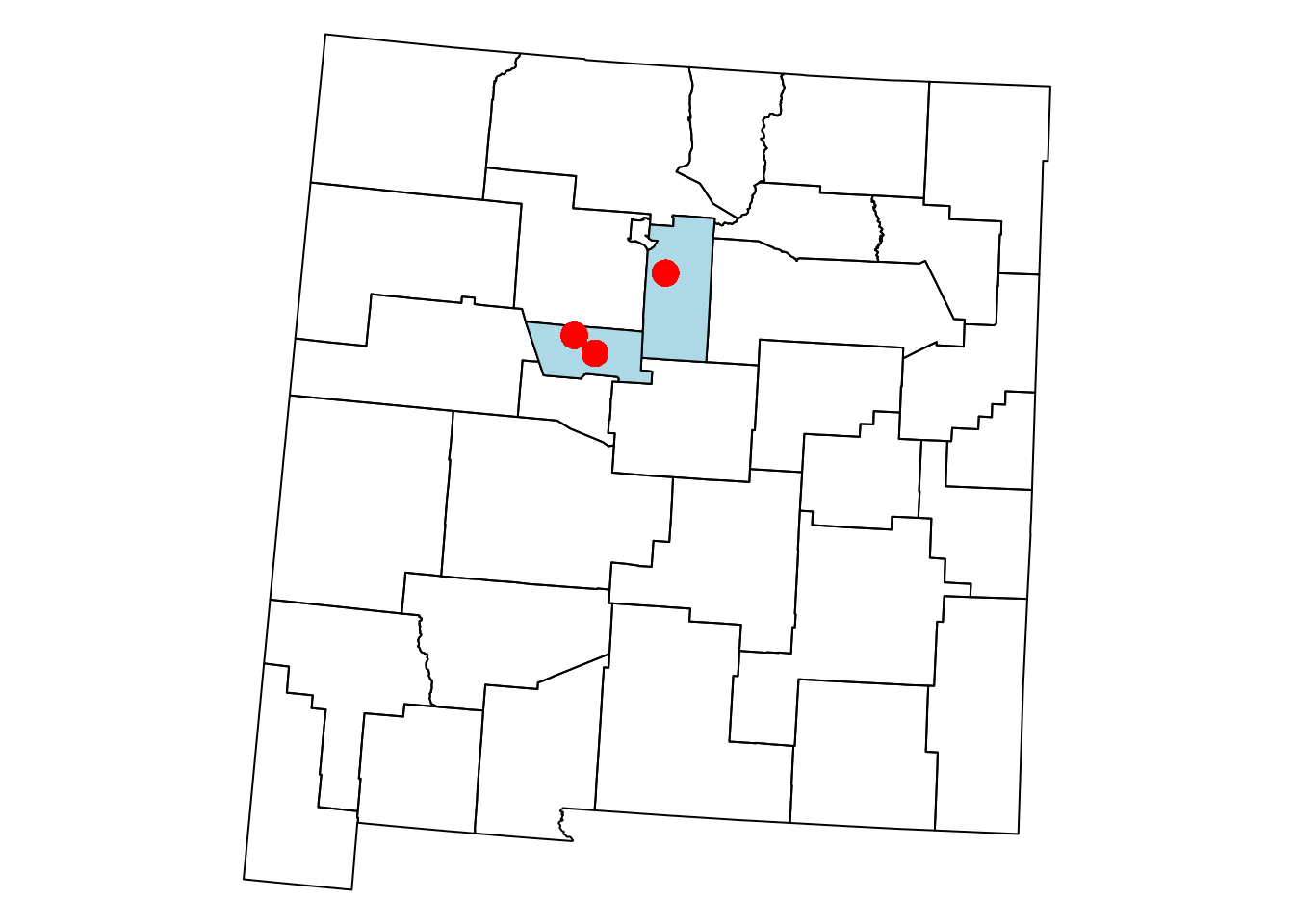

Figure 8.4: Subset of the nm layer based on intersection with airports

What will be the result of airports[nm,]?

What will be the result of nm[nm[20,],]?

8.3 Geometric calculations

8.3.1 Introduction

Geometric operations on vector layers can conceptually be divided into three groups, according to their output:

Numeric values (Section 8.3.2)—Functions that summarize geometrical properties of:
- A single layer—e.g., area, length (Section 8.3.2.2)
- A pair of layers—e.g., distance (Section 8.3.2.3)
Logical values (Section 8.3.3)—Functions that evaluate whether a certain condition holds true, regarding:
- A single layer—e.g., geometry is valid
- A pair of layers—e.g., feature A intersects feature B (Section 8.3.3)
Spatial layers (Section 8.3.4)—Functions that create a new layer based on:
- A single layer—e.g., centroid, buffer (Sections 8.3.4.2, 8.3.4.4, 8.3.4.5, 8.3.4.7)
- A pair of layers—e.g., intersection area (Section 8.3.4.6)

The following three sections elaborate and give examples of numeric (Section 8.3.2), logical (Section 8.3.3) and spatial (Section 8.3.4) geometric calculations on vector layers.

8.3.2 Numeric geometric calculations

8.3.2.1 Introduction

There are several functions to calculate numeric geometric properties of vector layers in package sf:

st_bbox—Section 7.5.2
st_area—Section 8.3.2.2
st_distance—Section 8.3.2.3
st_length—Section 11.4.6
st_dimension

Functions st_bbox, st_area, st_length, and st_dimension are applicable to individual geometries. The st_distance function is applicable to pairs of geometries. The next two sections give an example from each category: st_area for individual geometries (Section 8.3.2.2) and st_distance for pairs of geometries (Section 8.3.2.3).

8.3.2.2 Area

The st_area function returns the area of each feature or geometry. For example, we can use st_area to calculate the area of each feature in the county layer (i.e., each county):

county$area = st_area(county)
county$area[1:6]
## Units: [m^2]
## [1]  2455464324  1943957904  1079396694  1352486963 16439911090  2630547610

The result is an object of class units, which is basically a numeric vector associated with the units of measurement:

class(county$area)
## [1] "units"

CRS units (typically $m$ and $m^2$) are used by default in length, area and distance calculations. For example, the units of measurement in the US National Atlas CRS are meters, which is why the area values are returned in $m^2$ units. Calculations on layers in geographical CRS (i.e., lon/lat) are also returned in $m$ or $m^2$, even though—strictly speaking—the CRS units in such case are degrees. The mechanism which makes it possible is known as spherical geometry calculations, and it is provided by the s2 package.

We can convert units objects to different units, with set_units from package units³⁰. Note that the units package needs to be loaded to do that. For example, here is how we can convert the area column from $m^2$ to $km^2$:

library(units)
county$area = set_units(county$area, 'km^2')
county$area[1:6]
## Units: [km^2]
## [1]  2455.464  1943.958  1079.397  1352.487 16439.911  2630.548

Dealing with units, rather than numeric values has several advantages:

We don’t need to remember the coefficients for conversion between one unit to another, avoiding conversion mistakes.
We don’t need to remember, or somehow encode, the units of measurement (e.g., rename the area column to area_m2) since they are already binded with the values.
We can keep track of the units when making numeric calculations. For example, if we divide a numeric value by $km^2$, the result is going to be associated with units of density, $km^{-2}$ (Section 8.5).

Nevertheless, if we prefer to work with an ordinary numeric vector rather than a units vector, we can always make the conversion with as.numeric:

as.numeric(county$area[1:6])
## [1]  2455.464  1943.958  1079.397  1352.487 16439.911  2630.548

The calculated county area attribute values are visualized in Figure 8.5. Note that the pal argument can be used to specify the color scale, accepting either a fixed vector of color codes, or a function (such as here) to automatically generate an optimal number of colors:

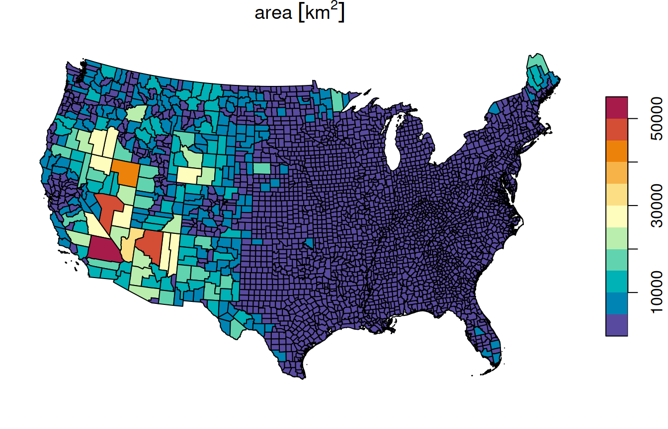
plot(county[, 'area'], pal = function(n) hcl.colors(n, 'Spectral', rev = TRUE))

Figure 8.5: Calculated area attribute of county

8.3.2.3 Distance

An example of a numeric operator on a pair of geometries is geographical distance. Keep in mind that geographical distance refers to shortest straight-line distance between the two given geometries. Distances can be calculated using function st_distance. For example, the following expression calculates the distances between each feature in airports and each feature in nm.

d = st_distance(airports, nm)

The result is a matrix of units values:

d[, 1:6]
## Units: [m]
##          [,1]     [,2]      [,3]      [,4]      [,5]      [,6]
## [1,] 267109.7 140421.5 103170.54 140823.90 175311.28 121918.82
## [2,] 276324.6 120820.7  93566.57 141502.56 177664.13 125392.75
## [3,] 197882.4 145824.8  34887.72  62177.71  96543.13  43650.59

In the distance matrix resulting from st_distance(x,y):

Rows refer to features of x, e.g., airports
Columns refer to features of y, e.g., nm

Therefore, the matrix dimensions are equal to c(nrow(x),nrow(y)):

c(nrow(airports), nrow(nm))
## [1]  3 33

dim(d)
## [1]  3 33

Just like areas (Section 8.3.2.2), distances can be converted to different units with set_units. For example, the following expression converts the distance matrix d from $m$ to $km$:

d = set_units(d, 'km')
d[, 1:6]
## Units: [km]
##          [,1]     [,2]      [,3]      [,4]      [,5]      [,6]
## [1,] 267.1097 140.4215 103.17054 140.82390 175.31128 121.91882
## [2,] 276.3246 120.8207  93.56657 141.50256 177.66413 125.39275
## [3,] 197.8824 145.8248  34.88772  62.17771  96.54313  43.65059

To work with the distance matrix, it can be convenient to set row and column names. We can use any of the unique attributes of x and y, such as airport names and county names:

rownames(d) = airports$name
colnames(d) = nm$NAME_2
d[, 1:6]
## Units: [km]
##                              Union San Juan Rio Arriba      Taos    Colfax
## Albuquerque International 267.1097 140.4215  103.17054 140.82390 175.31128
## Double Eagle II           276.3246 120.8207   93.56657 141.50256 177.66413
## Santa Fe Municipal        197.8824 145.8248   34.88772  62.17771  96.54313
##                                Mora
## Albuquerque International 121.91882
## Double Eagle II           125.39275
## Santa Fe Municipal         43.65059

Once row and column names are set, it can be more convenient to find out the distance between a specific airport and a specific county:

d['Santa Fe Municipal', 'Santa Fe', drop = FALSE]
## Units: [km]
##                    Santa Fe
## Santa Fe Municipal        0

8.3.3 Logical geometric calculations

Given two sets of geometries, or layers, x and y, the following logical geometric functions check whether each of the geometries in x maintains the specified relation with each of the geometries in y:

st_contains_properly
st_contains
st_covered_by
st_covers
st_crosses
st_disjoint
st_equals_exact
st_equals
st_intersects
st_is_within_distance
st_overlaps
st_touches
st_within

In this book we mostly use the st_intersects function, either

explicitly, i.e., executing st_intersects(x,y), or
implicitly, e.g., executing st_join (Section 8.1), or [ spatial subsetting (Section 8.2), which utilize st_intersects under the hood.

The st_intersects function detects intersection, which is the simplest and most useful type of relation: two geometries intersect when they share at least one point in common. However, it is important to be aware of the many other relations that can be evaluated using the other 12 functions.

By default, the above functions return a list, which takes less memory but is less convenient to work with. When specifying sparse=FALSE, the functions return a logical matrix which is more convenient to work with. The “logical relations” matrix is analogous to a distance matrix (Section 8.3.2.3). Each element i,j in the relations matrix is TRUE when f(x[i],y[j]) is TRUE.

For example, the following expression creates a matrix of intersection relations between counties in nm:

int = st_intersects(nm, nm, sparse = FALSE)
int[1:4, 1:4]
##       [,1]  [,2]  [,3]  [,4]
## [1,]  TRUE FALSE FALSE FALSE
## [2,] FALSE  TRUE  TRUE FALSE
## [3,] FALSE  TRUE  TRUE  TRUE
## [4,] FALSE FALSE  TRUE  TRUE

Figure 8.6 shows two matrices of spatial relations between counties in New Mexico: st_intersects (left) and st_touches (right).

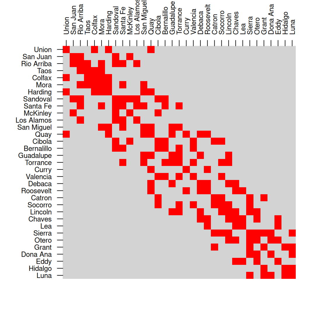
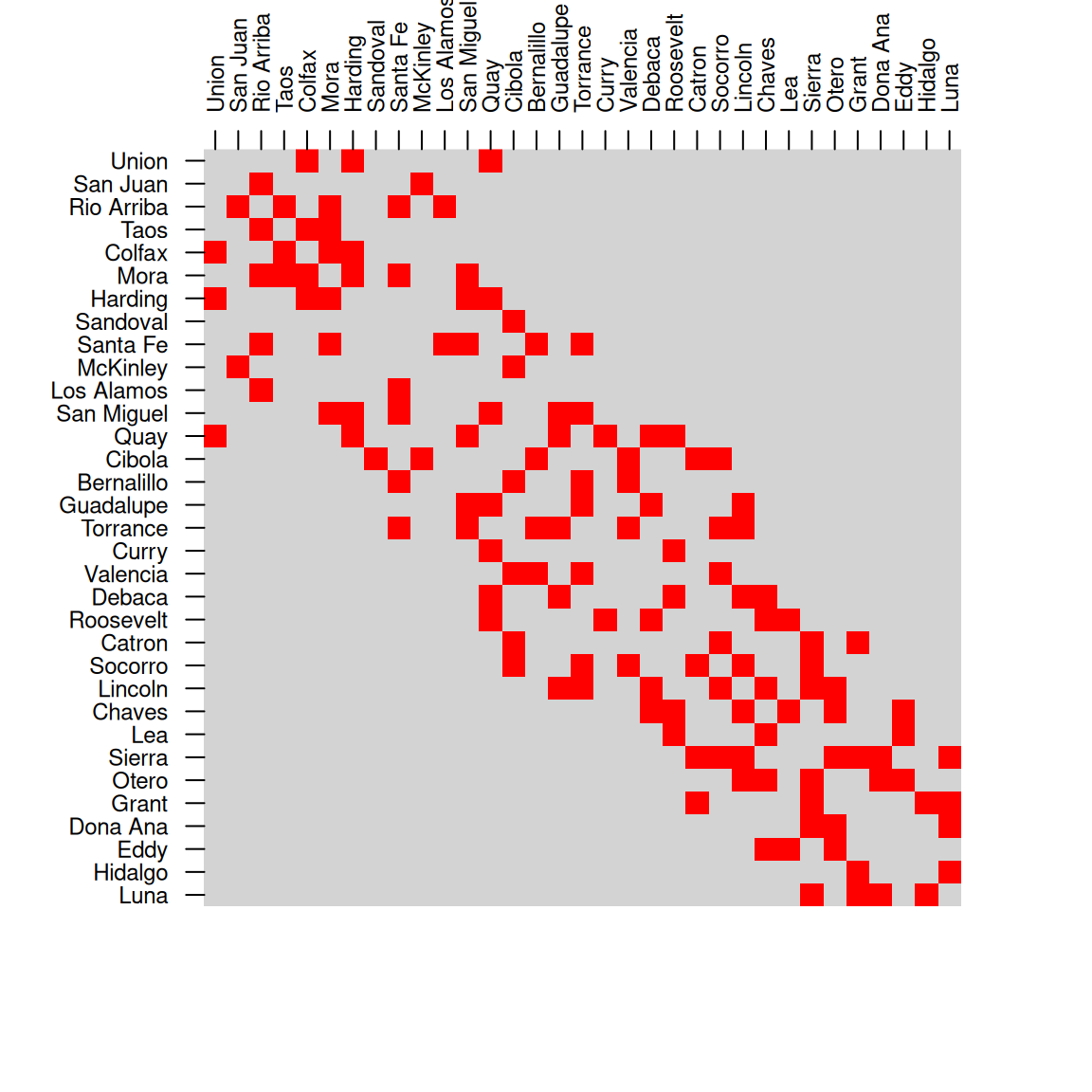
Figure 8.6: Spatial relations between counties in New Mexico, st_intersects (left) and st_touches (right)

How can we calculate airports count per county in nm, using st_intersects (Figure 8.7)?

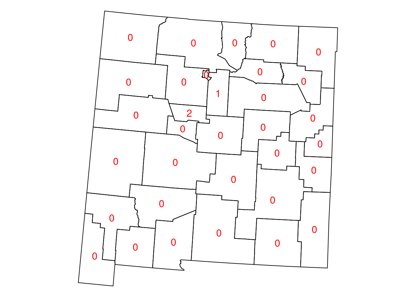
Figure 8.7: Airport count per county in New Mexico

8.3.4 Spatial geometric calculations

8.3.4.1 Introduction

The sf package provides common geometry-generating functions applicable to individual geometries, such as:

st_centroid—Section 8.3.4.2
st_buffer—Section 8.3.4.5
st_convex_hull—Section 8.3.4.7
st_voronoi
st_sample

What each function does is illustrated in Figure 8.8.

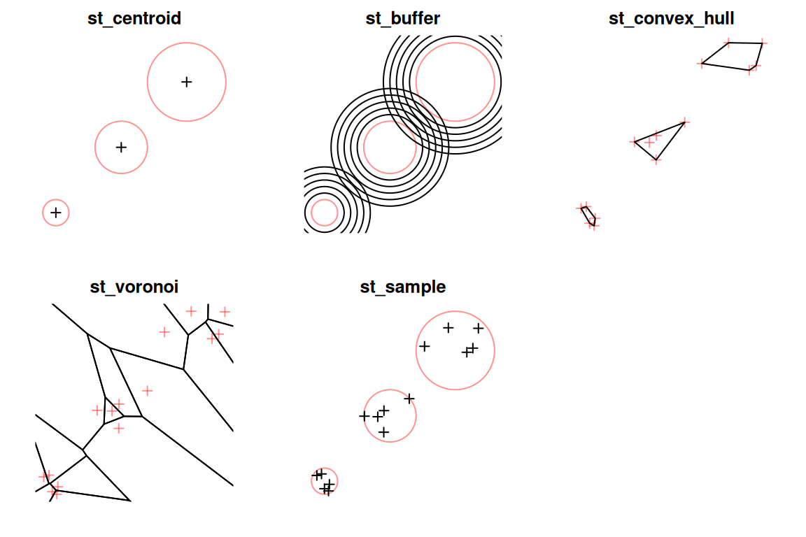
Figure 8.8: Geometry-generating operations on individual layers. The input geometries are shown in red, the output geometries are shown in black.

Additionally, the st_cast function is used to transform geometries from one type to another (Figure 7.6), which can also be considered as a sort of geometry generation (Section 8.3.4.4). The st_union and st_combine functions are used to combine multiple geometries into one, possibly dissolving their borders (Section 8.3.4.3).

Finally, geometry-generating functions which operate on pairs of geometries (Section 8.3.4.6) include:

st_intersection
st_difference
st_sym_difference
st_union

We elaborate on these functions in the following Sections 8.3.4.2–8.3.4.7.

8.3.4.2 Centroids

A centroid is the geometric center of a geometry, i.e., its center of mass, represented by a point. For example, the following expression uses st_centroid to create the centroid of each polygon in county:

ctr = st_centroid(nm)

The nm layer along with the calculated centroids is shown in Figure 8.9:

plot(st_geometry(nm), border = 'grey')
plot(st_geometry(ctr), col = 'red', pch = 3, add = TRUE)

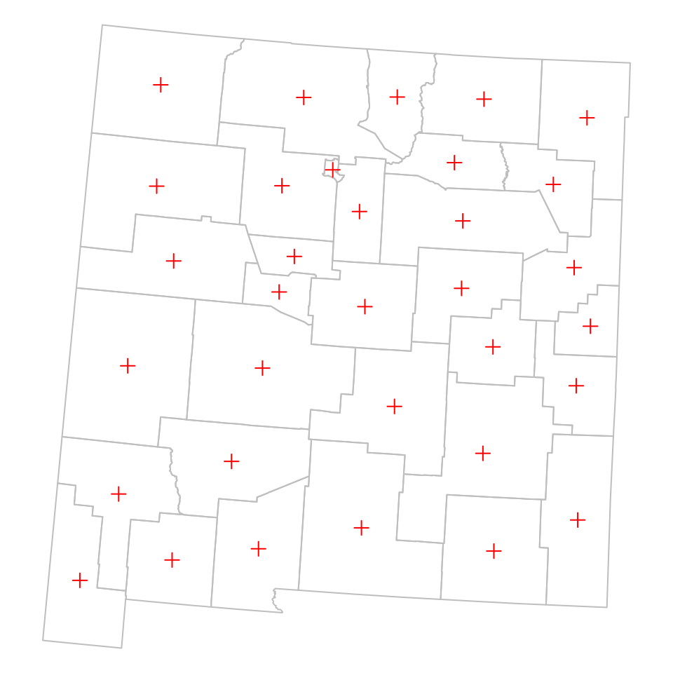
Figure 8.9: Centroids of New Mexico counties

8.3.4.3 Combining and dissolving

The st_combine and st_union functions can be used to combine multiple geometries into a single one. The difference is that st_combine only combines the geometries into one, just like the c function combines sfg objects into one sfg (Section 7.2.2), while st_union also dissolves internal borders.

To understand the difference between st_combine and st_union, let’s examine the result of applying each of them on nm:

st_combine(nm)
## Geometry set for 1 feature 
## Geometry type: MULTIPOLYGON
## Dimension:     XY
## Bounding box:  xmin: -865244.9 ymin: -1476219 xmax: -267619 ymax: -844629.9
## Projected CRS: NAD27 / US National Atlas Equal Area
## MULTIPOLYGON (((-267619 -883116.7, -267853.3 -8...

st_union(nm)
## Geometry set for 1 feature 
## Geometry type: POLYGON
## Dimension:     XY
## Bounding box:  xmin: -865244.9 ymin: -1476219 xmax: -267619 ymax: -844629.9
## Projected CRS: NAD27 / US National Atlas Equal Area
## POLYGON ((-850247.9 -1309181, -849518 -1301753,...

The results are plotted in Figure 8.10:

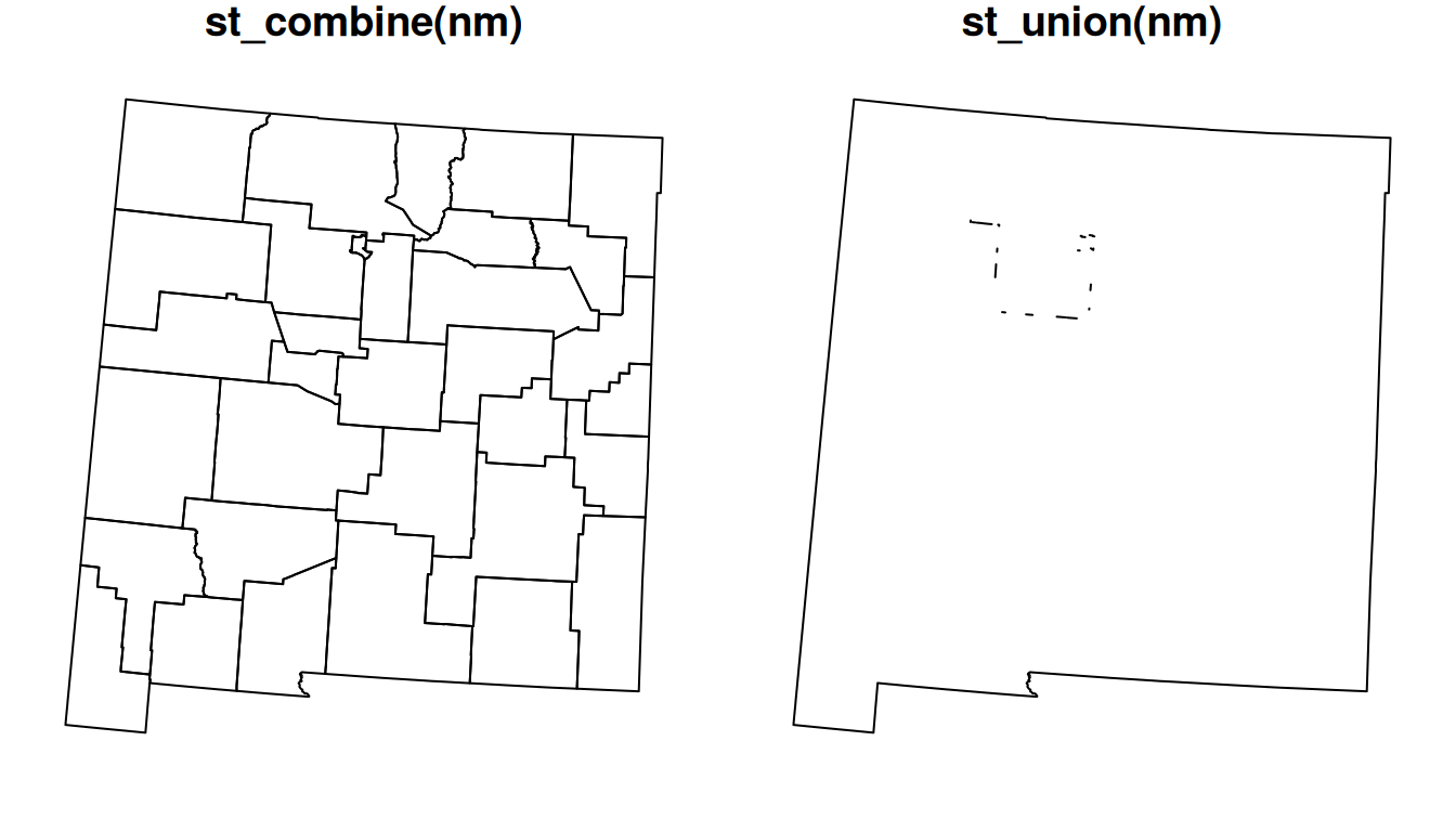
plot(st_combine(nm), main = 'st_combine(nm)')
plot(st_union(nm), main = 'st_union(nm)')

Figure 8.10: Combining (st_combine) and dissolving (st_union) polygons

What is the class of the resulting objects? Why? What happened to the original nm attributes?

Why did st_combine return a MULTIPOLYGON, while st_union returned a POLYGON?

Why do you think there are internal “patches” in the result of st_union(nm) (Figure 8.10)³¹?

Let’s solve a geometric question to practice some of the functions we learned so far. What is the distance between the centroids of California and New Jersey, in kilometers? Using [, st_union, st_centroid and st_distance, we can calculate the distance as follows:

# Subsetting
ca = county[county$NAME_1 == 'California', ]
nj = county[county$NAME_1 == 'New Jersey', ]

# Union
ca = st_union(ca)
nj = st_union(nj)

# Calculating centroids
ca_ctr = st_centroid(ca)
nj_ctr = st_centroid(nj)

# Calculating distance
d = st_distance(ca_ctr, nj_ctr)

# Converting to km
set_units(d, 'km')
## Units: [km]
##          [,1]
## [1,] 3855.579

Note that we are using st_union to combine the county polygons into a single geometry, so that we can calculate the centroid of the state polygon, as a whole.

To plot the centroids more conveniently, we can use the c function to combine two sfc (geometry columns) into one, long, geometry column. Recall that this is unlike what the c function does when given sfg (geometries), in which case the geometries are combined to one (multi- or collection) geometry (Section 7.2.2).

p = c(ca_ctr, nj_ctr)
p
## Geometry set for 2 features 
## Geometry type: POINT
## Dimension:     XY
## Bounding box:  xmin: -1711537 ymin: -666472.6 xmax: 2116465 ymax: -206156.2
## Projected CRS: NAD27 / US National Atlas Equal Area
## POINT (-1711537 -666472.6)
## POINT (2116465 -206156.2)

The centroids we calculated can be displayed as follows (Figure 8.11):

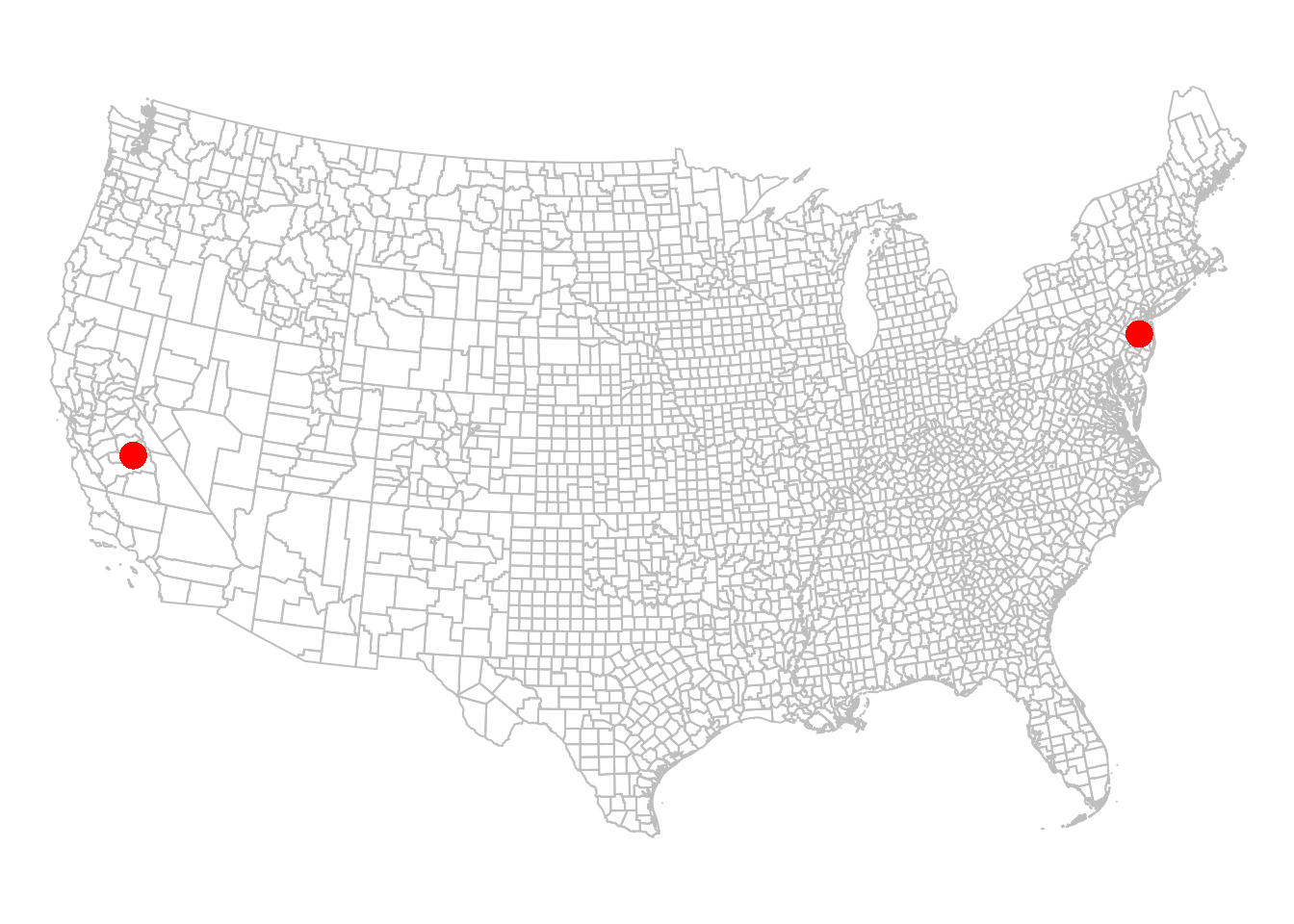
plot(st_geometry(county), border = 'grey')
plot(p, col = 'red', pch = 16, cex = 2, add = TRUE)

Figure 8.11: California and New Jersey centroids

How can we draw a line between the centroids, corresponding to the distance we just calculated (Figure 8.12)?

First, we can use st_combine to transform the points into a single MULTIPOINT geometry. Remember, the st_combine function is similar to st_union, but only combines and does not dissolve.

p = st_combine(p)
p
## Geometry set for 1 feature 
## Geometry type: MULTIPOINT
## Dimension:     XY
## Bounding box:  xmin: -1711537 ymin: -666472.6 xmax: 2116465 ymax: -206156.2
## Projected CRS: NAD27 / US National Atlas Equal Area
## MULTIPOINT ((-1711537 -666472.6), (2116465 -206...

Do you think the results of st_union(p) and st_combine(p) will be different, and if so in what way?

What is left to be done is to transform the MULTIPOINT geometry to a LINESTRING geometry, which is what we learn next (Section 8.3.4.4).

8.3.4.4 Geometry casting

Sometimes we need to convert a given geometry to a different type, to express different aspects of the geometries in our analysis. For example, we would have to convert the county MULTIPOLYGON geometries to MULTILINESTRING geometries to calculate the perimeter of each county, using st_length (Section 8.3.2).

The st_cast function can be used to convert between different geometry types. The st_cast function accepts:

The input sfg, sfc or sf
The target geometry type

For example, we can use st_cast to convert our MULTIPOINT geometry p (Figure 8.11), which we calculated in Section 8.3.4.3, to a LINESTRING geometry l:

l = st_cast(p, 'LINESTRING')
l
## Geometry set for 1 feature 
## Geometry type: LINESTRING
## Dimension:     XY
## Bounding box:  xmin: -1711537 ymin: -666472.6 xmax: 2116465 ymax: -206156.2
## Projected CRS: NAD27 / US National Atlas Equal Area
## LINESTRING (-1711537 -666472.6, 2116465 -206156.2)

Each MULTIPOINT geometry is replaced with a LINESTRING geometry, comprising a line that goes through all points from first to last. In this case, p contains just one MULTIPOINT geometry that contains two points. Therefore, the resulting geometry column l contains one LINESTRING geometry with a straight line.

The line we calculated is shown in Figure 8.12:

plot(st_geometry(county), border = 'grey')
plot(st_geometry(ca_ctr), col = 'red', pch = 16, cex = 2, add = TRUE)
plot(st_geometry(nj_ctr), col = 'red', pch = 16, cex = 2, add = TRUE)
plot(l, col = 'red', add = TRUE)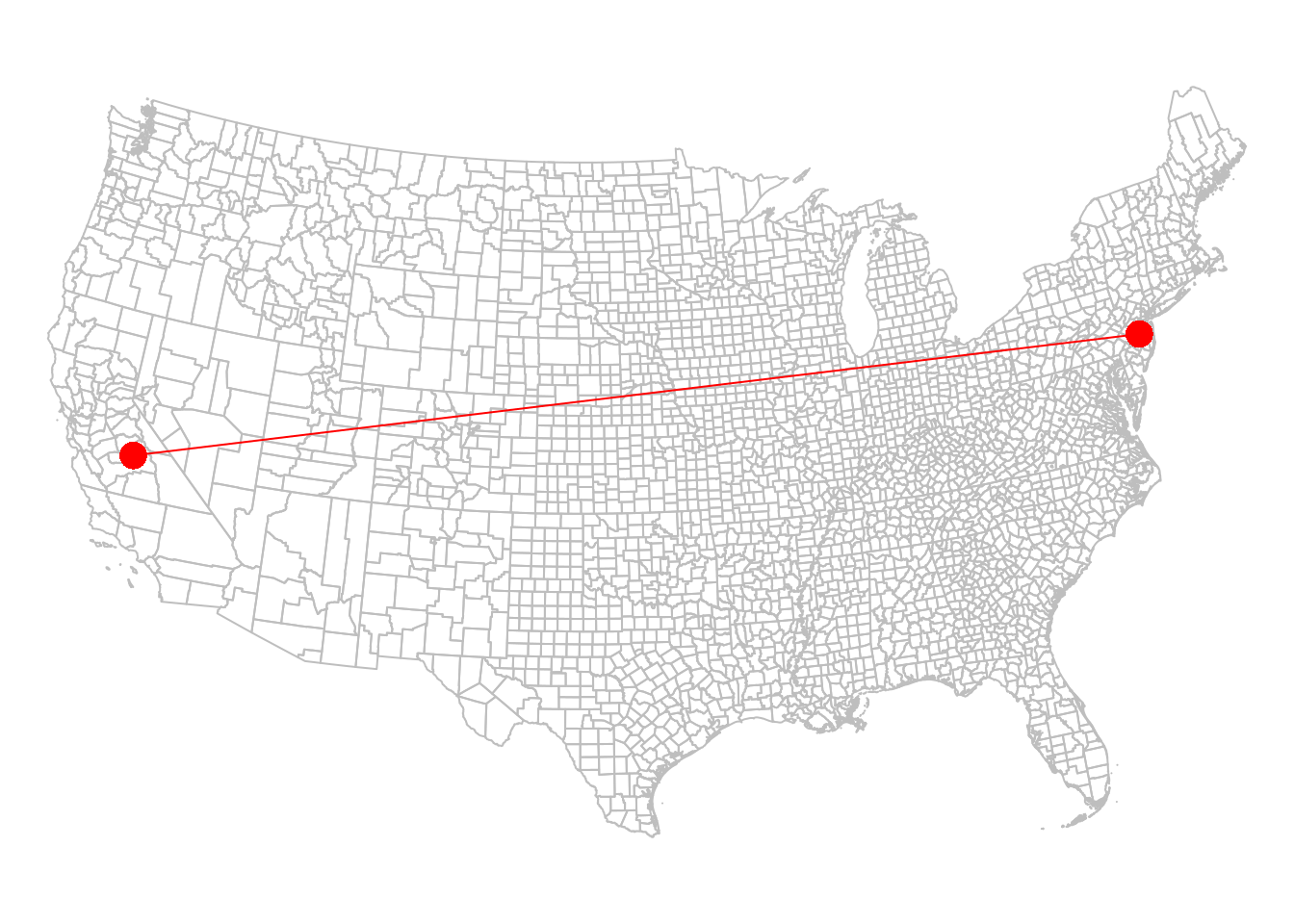

Figure 8.12: California and New Jersey centroids, with a line

It is worth mentioning that not every conversion operation between geometry types is possible. Meaningless st_cast operations will fail with an error message. For example, a LINESTRING composed of just two points cannot be converted to a POLYGON:

st_cast(l, 'POLYGON')
## Error in FUN(X[[i]], ...): polygons require at least 4 points

8.3.4.5 Buffers

Another example of a function that generates new geometries based on individual input geometries is st_buffer. The st_buffer function calculates buffers, polygons encompassing all points up to the specified distance from a given geometry.

For example, here is how we can calculate 100 $km$ buffers around the airports. Note that st_buffer requires buffer distance (dist), which can be passed as either:

numeric, in which case CRS units are assumed, or
units, in which case we can use any distance unit we wish.

The following two expressions are therefore equivalent, in both cases resulting in the same layer of 100 $km$ buffers named airports_100:

airports_100 = st_buffer(airports, dist = 100 * 10^3)

airports_100 = st_buffer(airports, dist = set_units(100, 'km'))

The airports_100 layer with the airport buffers is shown in Figure 8.13:

plot(st_geometry(nm))
plot(st_geometry(airports_100), add = TRUE)

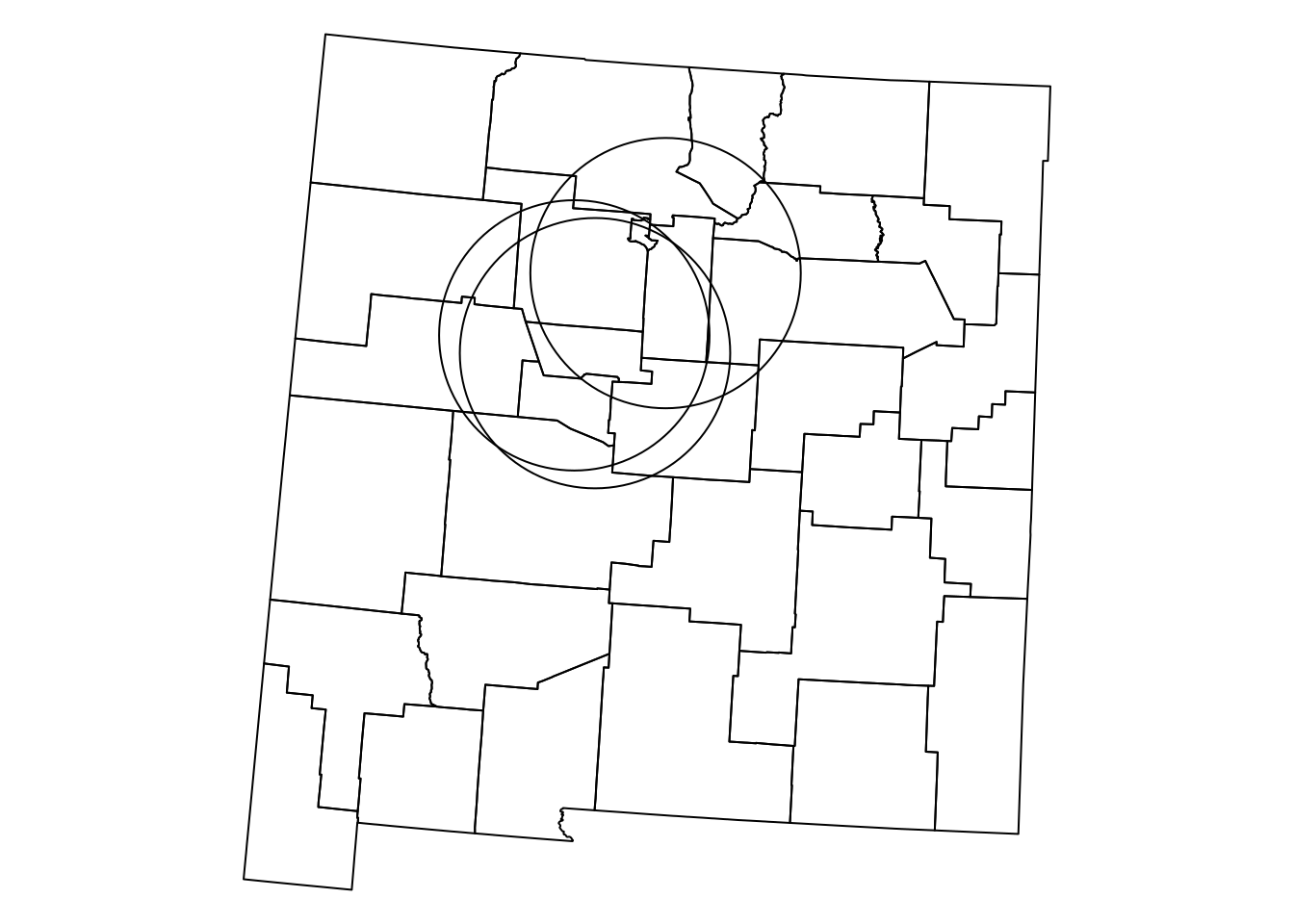
Figure 8.13: airports buffered by 100 km

8.3.4.6 Geometry generation from pairs

In addition to geometry-generating functions that operate on individual geometries, such as st_centroid (Section 8.3.4.2) and st_buffer (Section 8.3.4.5), there are four geometry-generating functions that operate on pairs of input geometries. These are:

st_intersection
st_difference
st_sym_difference
st_union

Figure 8.14 shows what each of these four functions does. Note that st_intersection, st_sym_difference, and st_union are symmetrical, meaning that the order of the two inputs does not matter, i.e., f(y,x) would return the same result as f(x,y). The st_difference function is not symmetrical: it returns the area of the first argument “minus” the area of the second, therefore f(y,x) would return a different result than f(x,y).

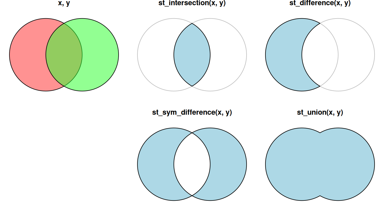
Figure 8.14: Geometry-generating operations on pairs of layers

For example, suppose that we need to calculate the area that is within 100 $km$ range of all three airports at the same time. We can find the area of intersection of the three airports, using st_intersection. Since st_intersection accepts two geometries at a time³², this can be done in two steps:

inter1 = st_intersection(airports_100[1, ], airports_100[2, ])
inter2 = st_intersection(inter1, airports_100[3, ])

The resulting polygon inter2 is shown, in blue, in Figure 8.15:

plot(st_geometry(nm))
plot(st_geometry(airports_100), add = TRUE)
plot(inter2, col = 'lightblue', add = TRUE)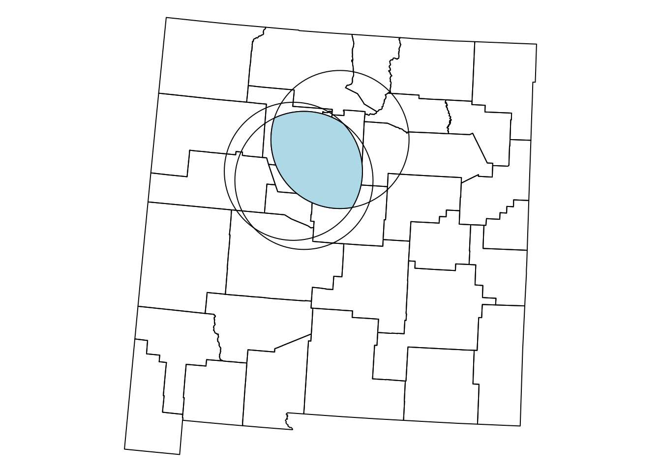

Figure 8.15: The intersection of three airports buffers

How can we calculate the area that is within 100 $km$ range of at least one of the three airports? We can use exactly the same technique, only replacing st_intersection with st_union, as follows:

union1 = st_union(airports_100[1, ], airports_100[2, ])
union2 = st_union(union1, airports_100[3, ])

As shown in Section 8.3.4.3, st_union can also be applied on an individual layer, in which case it returns the (dissolved) union of all geometries. Therefore we can get to the same result with just one expression, as follows:

union2 = st_union(airports_100)

The resulting polygon union2 is shown, in blue, in Figure 8.16:

plot(st_geometry(nm))
plot(union2, col = 'lightblue', add = TRUE)

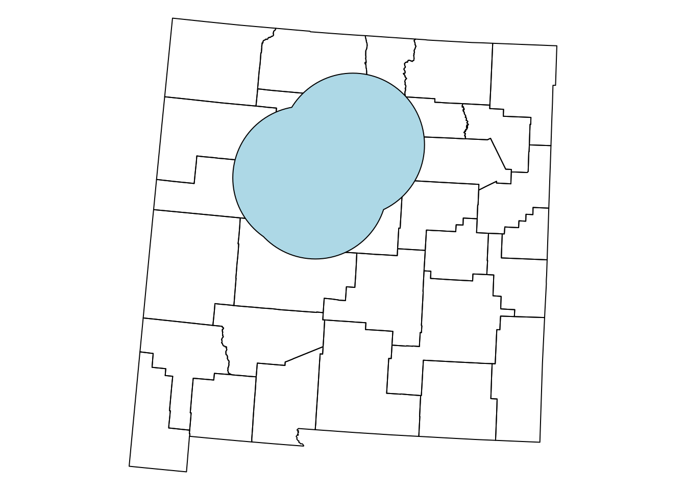
Figure 8.16: The union of three airports buffers

8.3.4.7 Convex hull

The Convex Hull of a set $X$ of points is the smallest convex polygon that contains $X$. The convex hull may be visualized as the shape resulting when stretching a rubber band around $X$, then releasing it until it shrinks to minimal size (Figure 8.17).

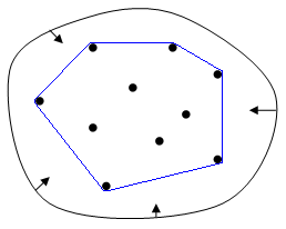
Figure 8.17: Convex Hull: elastic-band analogy (https://en.wikipedia.org/wiki/Convex_hull)

The st_convex_hull function is used to calculate the convex hull of the given geometry or geometries. For example, the following expression calculates the convex hull (per feature) in nm1:

h = st_convex_hull(nm1)

The resulting layer is shown in red in Figure 8.18:

plot(st_geometry(nm1))
plot(st_geometry(h), add = TRUE, border = 'red')

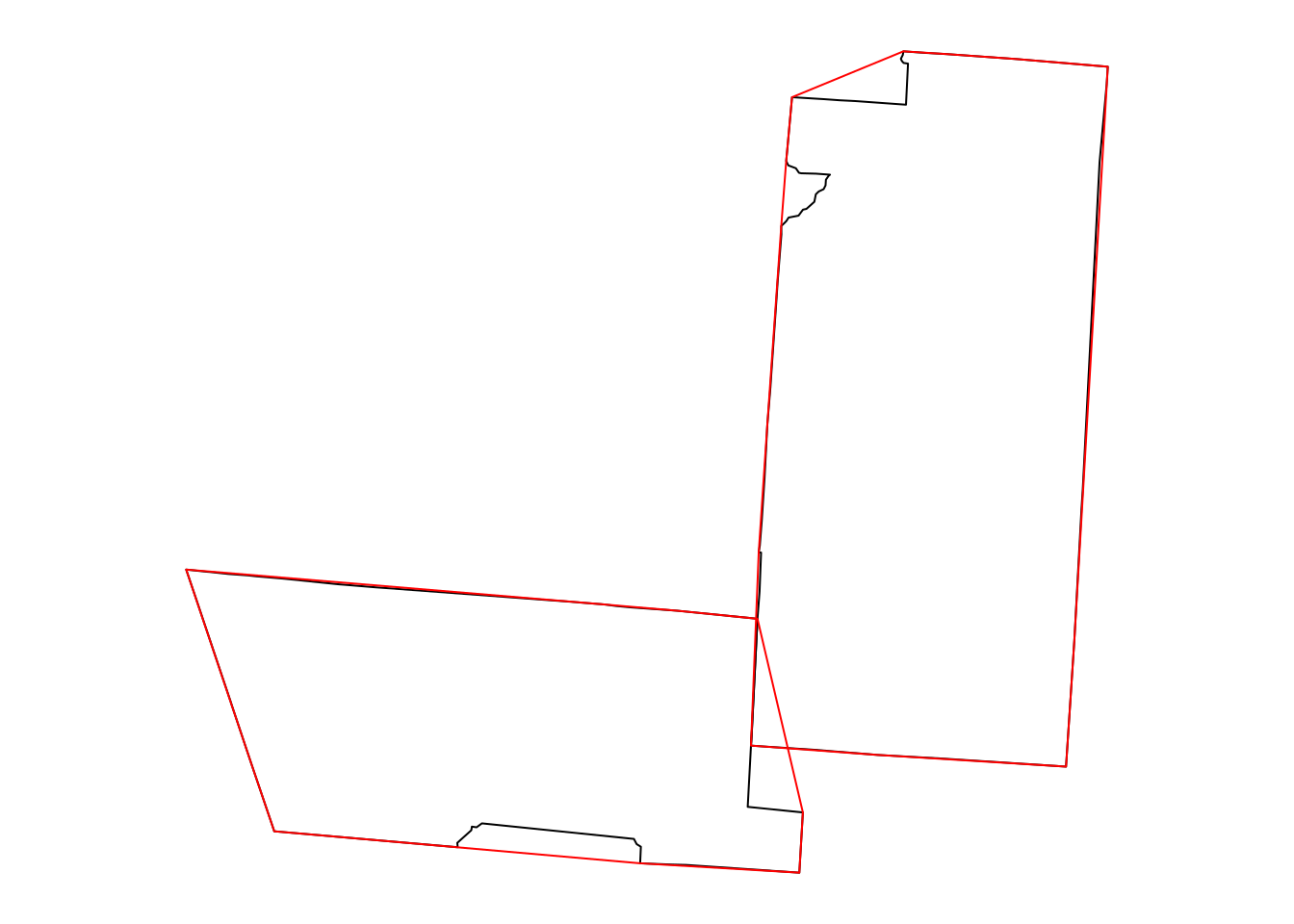
Figure 8.18: Convex hull polygons for two counties in New Mexico

How can we calculate the convex hull of all polygons in nm1 (Figure 8.19)?

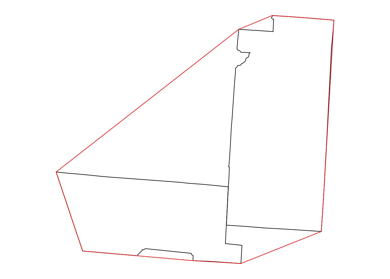
Figure 8.19: Convex Hull of multiple polygons

Here is another question to practice the geometric operations we learned in this chapter. Suppose we build a tunnel, 10 $km$ wide, between the centroids of 'Harding' and 'Sierra' counties in New Mexico. Which counties does the tunnel go through? The following code gives the result. Take a moment to go over it and make sure you understand what happens in each step:

w = nm[nm$NAME_2 %in% c('Harding', 'Sierra'), ]
w_ctr = st_centroid(w)
w_ctr_buf = st_buffer(w_ctr, dist = 5000)
w_ctr_buf_u = st_combine(w_ctr_buf)
w_ctr_buf_u_ch = st_convex_hull(w_ctr_buf_u)
nm_w = nm[w_ctr_buf_u_ch, ]
nm_w$NAME_2
## [1] "Harding"    "San Miguel" "Guadalupe"  "Torrance"   "Socorro"   
## [6] "Lincoln"    "Sierra"

Figure 8.20 shows the calculated tunnel geometry and highlights the counties that the tunnel goes through. The 4^th expression uses the text function to draw text labels. The text function accepts a matrix of coordinates specifying where labels should be drawn (e.g., county centroid coordinates), and the corresponding character vector of lables (e.g., county names). Note that in case the labels are numeric, such as in Figure 8.7, then we must convert them to character using as.character for them to be displayed using the text function.

plot(st_geometry(nm_w), border = NA, col = 'lightblue')
plot(st_geometry(nm), add = TRUE)
plot(st_geometry(w_ctr_buf_u_ch), add = TRUE)
text(st_coordinates(st_centroid(nm_w)), nm_w$NAME_2)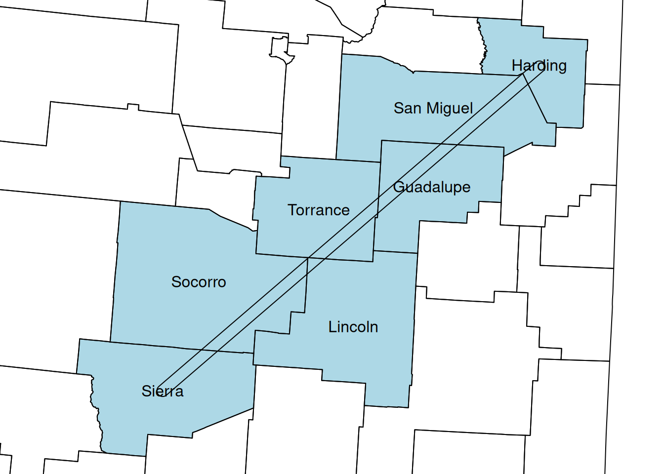

Figure 8.20: Tunnel between “Sierra” and “Harding” county centroids

How is the area of the “tunnel” divided between the various counties that it crosses? We can use st_intersection (Section 8.3.4.6) to calculate all pairwise intersections between the county polygons nm_w and the tunnel polygon w_ctr_buf_u_ch:

int = st_intersection(nm_w, w_ctr_buf_u_ch)
## Warning: attribute variables are assumed to be spatially constant throughout
## all geometries

The resulting layer int retains the attributes of the inputs. That way, we know which county each intersecting polygon belongs to:

int
## Simple feature collection with 7 features and 4 fields
## Geometry type: POLYGON
## Dimension:     XY
## Bounding box:  xmin: -678306.1 ymin: -1292072 xmax: -340822.6 ymax: -1001341
## Projected CRS: NAD27 / US National Atlas Equal Area
##          NAME_1     NAME_2 TYPE_2  FIPS                       geometry
## 1832 New Mexico    Harding County 35021 POLYGON ((-360222.7 -101210...
## 1843 New Mexico San Miguel County 35047 POLYGON ((-355700.3 -102139...
## 1858 New Mexico  Guadalupe County 35019 POLYGON ((-486351.8 -113244...
## 1863 New Mexico   Torrance County 35057 POLYGON ((-485590.3 -111976...
## 1878 New Mexico    Socorro County 35053 POLYGON ((-547660.2 -118141...
## 1887 New Mexico    Lincoln County 35027 POLYGON ((-547822 -1184777,...
## 1900 New Mexico     Sierra County 35051 POLYGON ((-637125.9 -125182...

Therefore, we can divide the area (Section 8.3.2.2) of each county intersection, by the total area of the tunnel, to get the proportion of tunnel area in each county:

int$area = st_area(int)
int
## Simple feature collection with 7 features and 5 fields
## Geometry type: POLYGON
## Dimension:     XY
## Bounding box:  xmin: -678306.1 ymin: -1292072 xmax: -340822.6 ymax: -1001341
## Projected CRS: NAD27 / US National Atlas Equal Area
##          NAME_1     NAME_2 TYPE_2  FIPS                       geometry
## 1832 New Mexico    Harding County 35021 POLYGON ((-360222.7 -101210...
## 1843 New Mexico San Miguel County 35047 POLYGON ((-355700.3 -102139...
## 1858 New Mexico  Guadalupe County 35019 POLYGON ((-486351.8 -113244...
## 1863 New Mexico   Torrance County 35057 POLYGON ((-485590.3 -111976...
## 1878 New Mexico    Socorro County 35053 POLYGON ((-547660.2 -118141...
## 1887 New Mexico    Lincoln County 35027 POLYGON ((-547822 -1184777,...
## 1900 New Mexico     Sierra County 35051 POLYGON ((-637125.9 -125182...
##                  area
## 1832  199091222 [m^2]
## 1843  872294022 [m^2]
## 1858  813570213 [m^2]
## 1863  702609547 [m^2]
## 1878 1119636195 [m^2]
## 1887  108029516 [m^2]
## 1900  575407772 [m^2]

int$prop = int$area / sum(int$area)
int
## Simple feature collection with 7 features and 6 fields
## Geometry type: POLYGON
## Dimension:     XY
## Bounding box:  xmin: -678306.1 ymin: -1292072 xmax: -340822.6 ymax: -1001341
## Projected CRS: NAD27 / US National Atlas Equal Area
##          NAME_1     NAME_2 TYPE_2  FIPS                       geometry
## 1832 New Mexico    Harding County 35021 POLYGON ((-360222.7 -101210...
## 1843 New Mexico San Miguel County 35047 POLYGON ((-355700.3 -102139...
## 1858 New Mexico  Guadalupe County 35019 POLYGON ((-486351.8 -113244...
## 1863 New Mexico   Torrance County 35057 POLYGON ((-485590.3 -111976...
## 1878 New Mexico    Socorro County 35053 POLYGON ((-547660.2 -118141...
## 1887 New Mexico    Lincoln County 35027 POLYGON ((-547822 -1184777,...
## 1900 New Mexico     Sierra County 35051 POLYGON ((-637125.9 -125182...
##                  area           prop
## 1832  199091222 [m^2] 0.04534448 [1]
## 1843  872294022 [m^2] 0.19867134 [1]
## 1858  813570213 [m^2] 0.18529656 [1]
## 1863  702609547 [m^2] 0.16002446 [1]
## 1878 1119636195 [m^2] 0.25500533 [1]
## 1887  108029516 [m^2] 0.02460451 [1]
## 1900  575407772 [m^2] 0.13105332 [1]

The proportions can be displayed as text labels, using the text function (Figure 8.21):

plot(st_geometry(nm_w), border = 'darkgrey')
plot(int, col = hcl.colors(nrow(int), 'Set3'), border = 'grey', add = TRUE)
text(st_coordinates(st_centroid(int)), paste0(round(int$prop, 2)*100, '%'))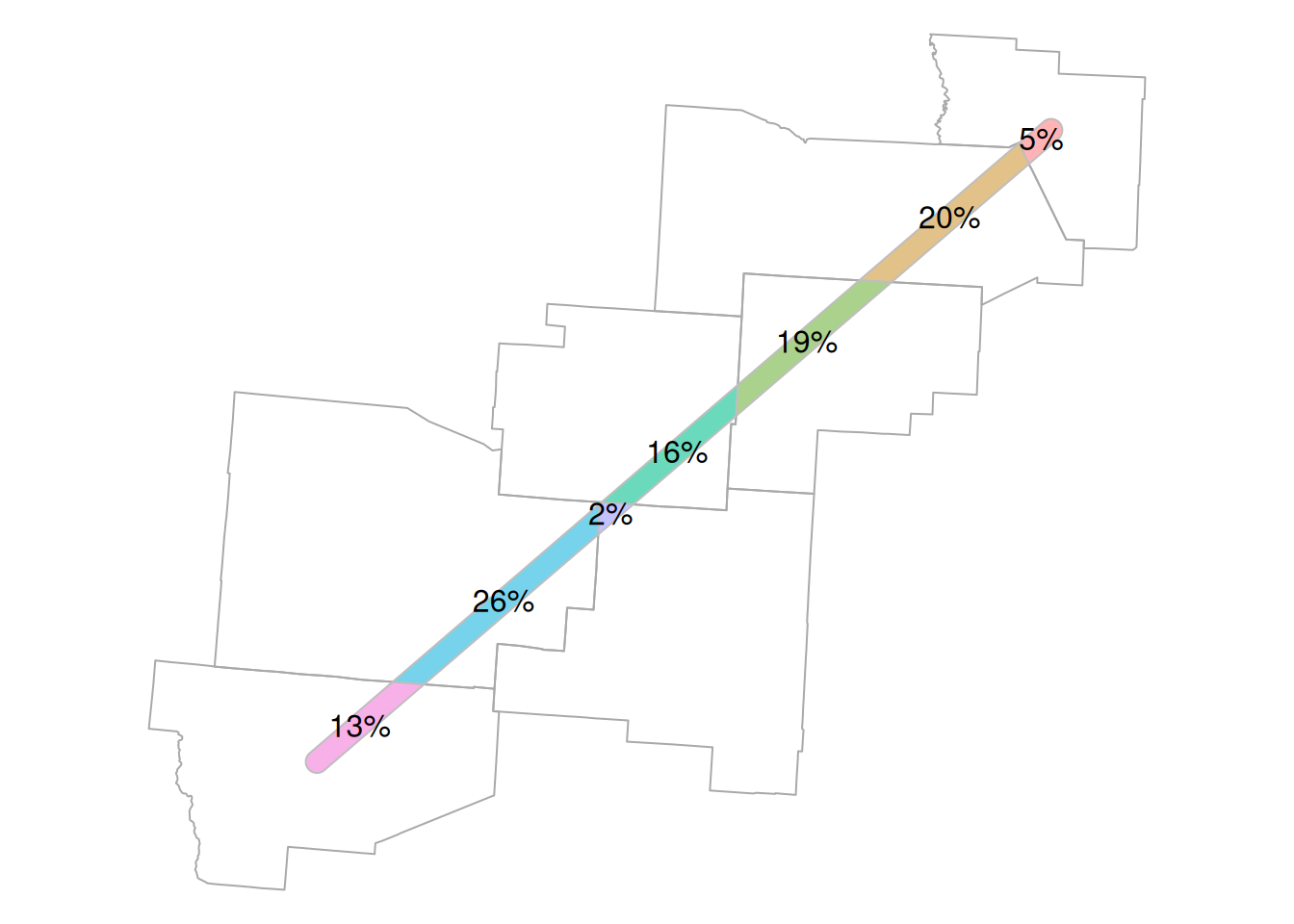

Figure 8.21: Proportion of tunnel area within each county

8.4 Vector layer aggregation

We don’t always want to dissolve all features into a single geometry (Section 8.3.4.3). Sometimes, we need to dissolve each group of geometries, whereas groups are specified by attribute or by location. To demonstrate dissolving by attribute, also known as aggregation, let’s take a subset of county with the counties of just four states: Arizona, Utah, Colorado, and New Mexico:

s = county[county$NAME_1 %in% c('Arizona', 'Utah', 'Colorado', 'New Mexico'), ]

The selected counties are shown in Figure 8.22:

plot(s[, 'NAME_1'], key.pos = 4, key.width = lcm(4))

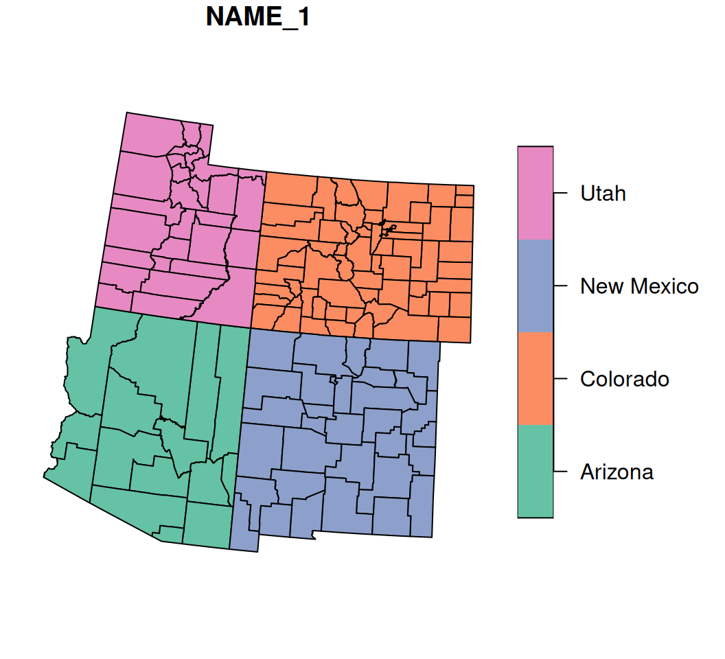
Figure 8.22: Subset of four states from county

As shown previously (Section 8.3.4.3), we can dissolve all features into a single geometry with st_union:

s1 = st_union(s)
s1
## Geometry set for 1 feature 
## Geometry type: POLYGON
## Dimension:     XY
## Bounding box:  xmin: -1391613 ymin: -1476219 xmax: -172543.1 ymax: -234961.4
## Projected CRS: NAD27 / US National Atlas Equal Area
## POLYGON ((-887019.2 -1466057, -895485.9 -146515...

The dissolved geometry is shown in Figure 8.23:

plot(s1)

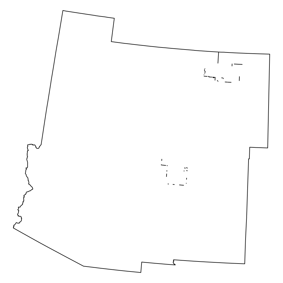
Figure 8.23: Union of all counties in s

Alternatively, we can aggregate/dissolve by attributes, using the aggregate function³³. aggregate accepts the following arguments:

x—The sf layer being dissolved
by—A corresponding data.frame determining the groups
FUN—The function to be applied on each attribute in x

For example, the following expression dissolves the layer s, summing the area attribute, by state:

s2 = aggregate(s[, 'area'], st_drop_geometry(s[, 'NAME_1']), sum)
s2
## Simple feature collection with 4 features and 2 fields
## Attribute-geometry relationships: aggregate (1), identity (1)
## Geometry type: POLYGON
## Dimension:     XY
## Bounding box:  xmin: -1391613 ymin: -1476219 xmax: -172543.1 ymax: -234961.4
## Projected CRS: NAD27 / US National Atlas Equal Area
##       NAME_1            area                       geometry
## 1    Arizona 295352.1 [km^2] POLYGON ((-1087751 -1430224...
## 2   Colorado 269731.2 [km^2] POLYGON ((-521848 -869940.6...
## 3 New Mexico 314871.3 [km^2] POLYGON ((-850247.9 -130918...
## 4       Utah 219829.9 [km^2] POLYGON ((-1015168 -818312....

The result is shown in Figure 8.24:

plot(s2[, 'area'], key.pos = 4)

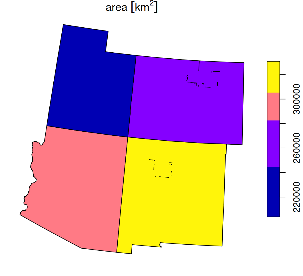
Figure 8.24: Union by state name of s

8.5 Join by attributes

Attaching new attributes to a vector layer from a table, based on common attribute(s), is known as a non-spatial join, or join by attributes. Joining by attributes works exactly the same way as a join between two tables, e.g., using the merge function (Section 4.6). The difference is just that the “left” table, x, is an sf layer, instead of a data.frame. Using merge to join an sf layer with a data.frame is analogous to the “Join attributes from a table” workflow in ArcGIS (Figure 8.25).

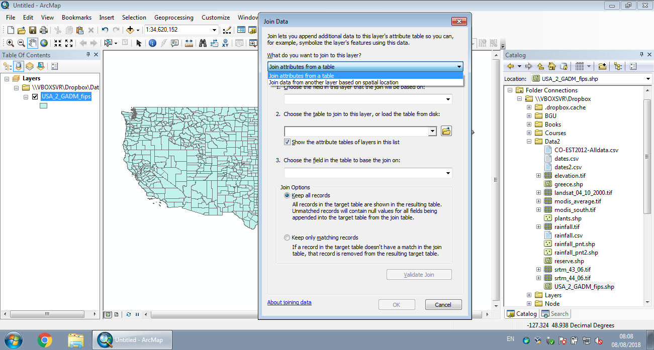
Figure 8.25: Join by attributes in ArcGIS

In the next example we will join county-level demographic data, from CO-EST2012-Alldata.csv, with the county layer. The join will be based on the common Federal Information Processing Standards (FIPS) code of each county.

First, let’s read the CO-EST2012-Alldata.csv file into a data.frame named dat. This file contains numerous demographic variables, on the county level, in the US:

dat = read.csv('data/CO-EST2012-Alldata.csv')

Next, we subset the columns we are interested in, so that it is easier to display the table:

STATE—State code
COUNTY—County code
CENSUS2010POP—Population size in 2010

The first two columns, STATE and COUNTY, contain the state and county components of the FIPS code, which we will use to join the data. The third column, CENSUS2010POP, contains our variable of interest, which we want to attach to the county layer.

dat = dat[, c('STATE', 'COUNTY', 'CENSUS2010POP')]
head(dat)
##   STATE COUNTY CENSUS2010POP
## 1     1      0       4779736
## 2     1      1         54571
## 3     1      3        182265
## 4     1      5         27457
## 5     1      7         22915
## 6     1      9         57322

Records where COUNTY code is 0 are state sums, i.e. sub-totals. We need to remove the state sums and keep just the county-level records:

dat = dat[dat$COUNTY != 0, ]
head(dat)
##   STATE COUNTY CENSUS2010POP
## 2     1      1         54571
## 3     1      3        182265
## 4     1      5         27457
## 5     1      7         22915
## 6     1      9         57322
## 7     1     11         10914

The FIPS code in the county layer is a character value with five digits, where the first two digits are the state code and the last three digits are the county code. When necessary, leading zeros are added. For example, state code 9 and county code 5 is encoded as '09005'.

county$FIPS[1:6]
## [1] "09005" "09003" "09013" "09015" "06093" "06015"

The table dat, however, contains state and county coded as separate numeric values:

dat$STATE[1:10]
##  [1] 1 1 1 1 1 1 1 1 1 1

dat$COUNTY[1:10]
##  [1]  1  3  5  7  9 11 13 15 17 19

To join county with dat, we need either to “split” the FIPS codes in county into two separate numeric columns (as in dat), or to “paste” the separate columns in dat into one column with 5-digit codes (as in county). We will demonstrate the latter.

To create a single columns with county FIPS codes, in dat, we need to:

Standardize the state code to a two-digit code
Standardize the county code to three-digit code
Paste the state code and the county code, to obtain the five-digit FIPS code

The formatC function can be used to format numeric values into different formats, using different “scenarios”. The “add leading zeros” scenario is specified using width=n, where n is the required number of digits, and flag='0'. Therefore:

dat$STATE = formatC(dat$STATE, width = 2, flag = '0')
dat$COUNTY = formatC(dat$COUNTY, width = 3, flag = '0')
dat$FIPS = paste0(dat$STATE, dat$COUNTY)

The STATE and COUNTY columns are no longer necessary and can be dropped:

dat$STATE = NULL
dat$COUNTY = NULL

Now we have a column named FIPS, with FIPS codes in exactly the same format as in the county layer:

head(dat)
##   CENSUS2010POP  FIPS
## 2         54571 01001
## 3        182265 01003
## 4         27457 01005
## 5         22915 01007
## 6         57322 01009
## 7         10914 01011

This means we can join the county layer with the dat table, based on the common column named FIPS, as follows:

county = merge(county, dat, by = 'FIPS', all.x = TRUE)
county
## Simple feature collection with 3103 features and 6 fields
## Geometry type: MULTIPOLYGON
## Dimension:     XY
## Bounding box:  xmin: -2036899 ymin: -2112691 xmax: 2523822 ymax: 732063.4
## Projected CRS: NAD27 / US National Atlas Equal Area
## First 10 features:
##     FIPS  NAME_1   NAME_2 TYPE_2            area CENSUS2010POP
## 1  01001 Alabama  Autauga County 1561.848 [km^2]         54571
## 2  01003 Alabama  Baldwin County 4243.393 [km^2]        182265
## 3  01005 Alabama  Barbour County 2328.395 [km^2]         27457
## 4  01007 Alabama     Bibb County 1620.534 [km^2]         22915
## 5  01009 Alabama   Blount County 1691.582 [km^2]         57322
## 6  01011 Alabama  Bullock County 1622.805 [km^2]         10914
## 7  01013 Alabama   Butler County 2011.518 [km^2]         20947
## 8  01015 Alabama  Calhoun County 1590.532 [km^2]        118572
## 9  01017 Alabama Chambers County 1556.228 [km^2]         34215
## 10 01019 Alabama Cherokee County 1549.377 [km^2]         25989
##                          geometry
## 1  MULTIPOLYGON (((1228285 -12...
## 2  MULTIPOLYGON (((1202321 -15...
## 3  MULTIPOLYGON (((1410753 -13...
## 4  MULTIPOLYGON (((1209412 -12...
## 5  MULTIPOLYGON (((1262686 -11...
## 6  MULTIPOLYGON (((1373074 -12...
## 7  MULTIPOLYGON (((1282594 -13...
## 8  MULTIPOLYGON (((1316304 -11...
## 9  MULTIPOLYGON (((1377074 -11...
## 10 MULTIPOLYGON (((1336060 -10...

Note that we are using a left join, therefore the county layer retains all of its records, whether or not there is a match in the dat table (Section 4.6.2). Features in county that do not have a matching FIPS value in dat get NA in the new CENSUS2010POP column.

A map of the new CENSUS2010POP attribute, using the default equal breaks, is shown in Figure 8.26:

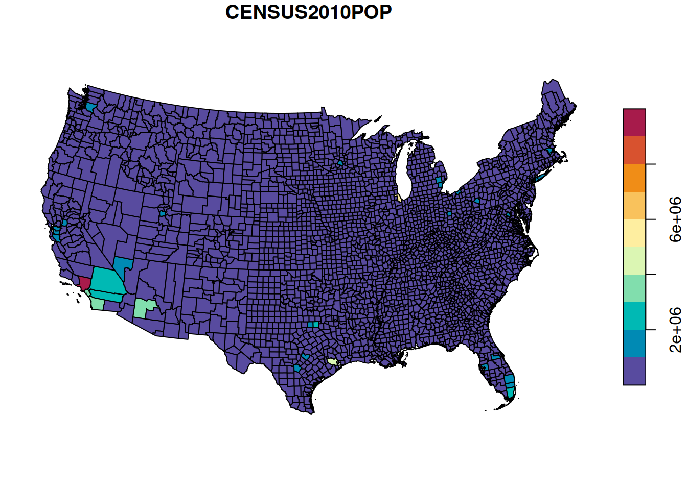
plot(county[, 'CENSUS2010POP'], pal = function(n) hcl.colors(n, 'Spectral', rev = TRUE))

Figure 8.26: Population size per county in the US (equal breaks)

Almost all counties fall into the first category, therefore the map is uniformely colored and not very informative. A map using quantile breaks (Figure 8.27) reveals the spatial pattern of population sizes more clearly:

plot(county[, 'CENSUS2010POP'], breaks = 'quantile', pal = function(n) hcl.colors(n, 'Spectral', rev = TRUE))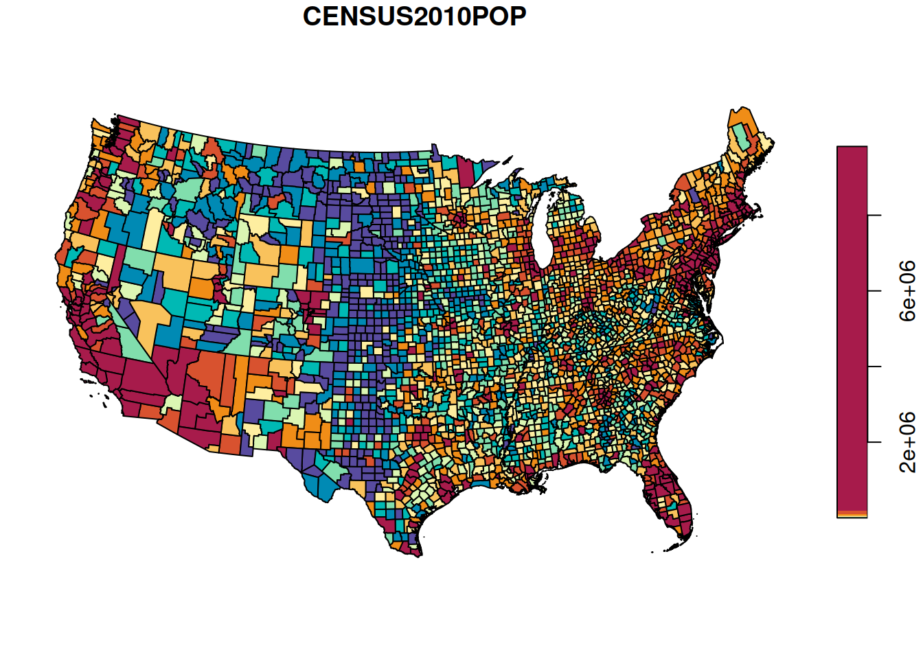

Figure 8.27: Population size per county in the US (quantile breaks)

Another issue with the map is that county population size also depends on county area, which can make the pattern misleading in case when county area sizes are unequal (which they are). To safely compare the counties we need to standardize population size by county area. In other words, we need to calculate population density:

county$density = county$CENSUS2010POP / county$area

Note how the measurement units ($km^{-2}$, i.e., number of people per $km^2$) for the new column are automatically determined based on the inputs:

head(county$density)
## Units: [1/km^2]
## [1] 34.940025 42.952659 11.792244 14.140402 33.886615  6.725391

The map of population densities per county is shown in Figure 8.28:

plot(county[, 'density'], breaks = 'quantile', pal = function(n) hcl.colors(n, 'Spectral', rev = TRUE))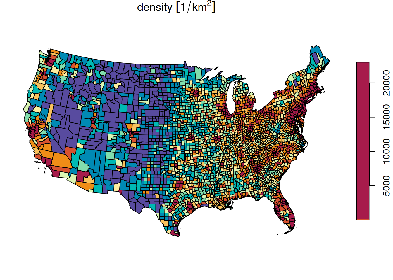

Figure 8.28: Population density in the US, quantile breaks

How many features in county did not have a matching FIPS code in dat? What are their names?

How many features in dat do not have a matching FIPS code in county?

We can also calculate the average population density in the US, by dividing the total population by the total area:

sum(county$CENSUS2010POP, na.rm = TRUE) / sum(county$area)
## 39.19633 [1/km^2]

This is close to the population density in 2010 according to Wikipedia, which is 40.015.

Simply averaging the density column gives an overestimation, because all counties get equal weight while in reality the smaller counties are more dense:

mean(county$density, na.rm = TRUE)
## 93.80553 [1/km^2]

8.6 Recap: main data structures

Table 8.1 summarizes the main data structures we learn in this book.

Table 8.1: Main data structures in the book
Chapter	Category	Class
2	Vector	`numeric`, `character`, `logical`
3	Date	`Date`
4	Table	`data.frame`
5	Matrix	`matrix`
5	Array	`array`
5	Raster	`stars`
7	Vector layer	`sfg`, `sfc`, `sf`
8	Units	`units`
11	List	`list`
12	Geostatistical model	`gstat`
12	Variogram model	`variogramModel`

Use valid_udunits() to see the list of available units.↩︎
To avoid these “patches”, we can reduce the precision of the calculation using function st_set_precision. For example, compare the plot of st_union(st_set_precision(nm, units::set_units(1,'mm'))) with the plot of st_union(nm) (Figure 8.10) (https://r-spatial.org/book/03-Geometries.html#sec-precision).↩︎
st_intersection has another mode of operation on an individual layer. Check out the code x=st_intersection(airports_100);x[x$n.overlaps==nrow(airports_100),].↩︎
The group_by and summarize functions from package dplyr can also be used for aggregation, instead of aggregate: s2 = s |> group_by(NAME_1) |> summarize(area = sum(area)).↩︎