Chapter 1 The R environment

Last updated: 2024-03-20 11:43:39

Aims

Our aims in this chapter are:

• Introduce general concepts of programming languages
• Introduce the R environment
• Learn to write and execute basic expressions in R

1.1 Programming

1.1.1 What is programming?

A computer program is a sequence of text instructions that can be “understood” by a computer and executed. A programming language is a machine-readable artificial language designed to express computations that can be performed by a computer. Programming is the preferred way for giving instructions to the computer, because that way:

• we break free from the limitations of the graphical interface, and are able to perform tasks that are unfeasible or even impossible, and
• we can keep the code for editing and re-use in the future, and as a reminder to ourselves of what we did in the past, and share a precise record of our analysis with others, making our results reproducible.

1.1.2 Computer hardware

When learning programming in R, at times we will refer to specific components of the computer hardware to describe what is going on “behind the scenes”. For now, here is a summary of the main computer hardware components (Figure 1.1.2):

• The Central Processing Unit (CPU)—This is where the actual computation takes place. The CPU performs (simple) calculations, very fast.
• The Random Access Memory (RAM)—Short-term fast memory, where the objects and variables we are working with are stored. The RAM is cleared each time we turn off the computer.
• Mass Storage (e.g., hard drive)—Long-term and high-capacity slow memory, where data—such as code files, spreadsheets, spatial layers, etc.—are stored persistently. Examples of mass storage are hard drives and USB flash drives. The contents of mass storage devices persists even when the computer is turned off.
• A Keyboard—This is an example of an input device, which we use to give instructions to the computer.
• A Screen—This is an example of an output device, were we can see the results returned by the computer. Another example of an output device is a printer.
• The Network—Access to the internet network makes it possible to obtain data from other computers, and to share our code and results.

Figure 1.1: Components of a computing environment

Importantly, we will see that working with a programming language involves (at least) the CPU and RAM. The CPU is where calculations, such as arithmetic (Section 1.3.2), are being done. The RAM is where we store the inputs and the results of those calculations (Section 2.2). The input (e.g., keyboard) and output (e.g., screen) devices may be used to enter the instructions to the computer (in the form of computer code), and to examine the results, respectively. Mass storage devices (e.g., hard drive) are used to presistently store information, such as the code and its results. Finally, the network also makes it easy to share our code and data with others, as well as to obtain software, such as the R software (Section 1.2) and R packages (Section 5.3.3).

Next, we introduce four central concepts of programming in general, and programming in R in particular:

• Abstraction (Section 1.1.3)
• Execution models (Section 1.1.3)
• Object-oriented programming (Section 1.1.4)
• Inheritance (Section 1.1.5).

Afterwards, we move on to introduce the R software and environment (Section 1.2) and actually writing R code (Section 1.3).

1.1.3 Abstraction and execution models

Programming languages differ in two main aspects: their level of abstraction and their execution models. Abstraction is the presentation of data and instructions which hide implementation details. Abstraction is what lets the programmer focus on the task at hand, ignoring the small technical details (Figure 1.2).

Low-level programming languages provide little or no abstraction. The advantage of low-level programming languages is their efficient memory use and therefore fast execution. Their disadvantage is that they are relatively difficult to use, because of the many technical details that the programmer needs to know, even to do simple tasks.

High-level programming languages provide more abstraction and automatically handle various aspects, such as memory use. The advantage of high-level languages is that they are more “understandable”, therefore easier to use. The disadvantage is that high-level languages can be less efficient and therefore slower.

Figure 1.2: Code to print a text message (“Hello World”), using Assembly, C++, and R programming languages. We can see the increasing abstraction, and code simplicity, among the languages, from left to right.

For most practical purposes, the convenience of working with high-level languages greatly outweights their somewhat lower performance in terms of speed. This is why, at present, high-level languages are widely used for almost all purposes (including working with spatial data), while low-level languages are reserved for tasks where performance is critical, such as operating systems, computer games, etc. The R language, which we are using in this book, is a high-level programming language.

Execution models are systems for execution of programs written in a given programming language. In compiled execution models, before being executed the code needs to be compiled into executable machine code. In compiled execution models, the code is first translated to an executable file (Figure 1.3). Subsequently, the executable file can then be run (Figure 1.4). In interpreted execution models, the code can be run directly, using the interpreter (Figure 1.5). The advantage of the interpretation approach is that it is easier to develop and use the language. The disadvantage, again, is lower efficiency.

Figure 1.3: Compilation of C++ code

Figure 1.4: Running an executable file

Figure 1.5: Running R code

Just like with abstraction levels, the convenience of working with interpreted languages usually outweights the gain in performance of compiled languages. Therefore, the former are preferable for most practical purposes. R—along with Python, and many other languages—belongs in the group of high-level interpreted languages (Figure 1.6).

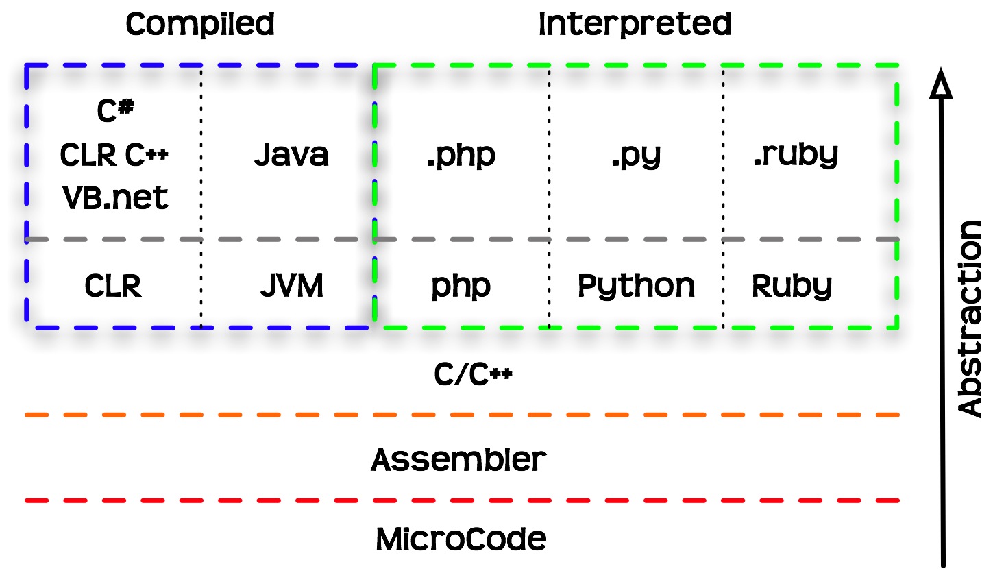
Figure 1.6: Programming languages classified based on abstraction levels and execution models

1.1.4 Object-oriented programming

In object-oriented programming, the interaction with the computer takes places through objects. Each object belongs to a class: an abstract structure with certain properties. Objects are in fact instances of a class.

The class comprises a template which sets the properties and methods each object of that class should have, while an object contains specific values for that particular instance (Figure 1.7).

For example:

• All cars we see in the parking lot are instances of the “car” class
• The “car” class has certain properties (manufacturer, color, year) and methods (start, drive, stop)
• Each “car” object has specific values for the properties (Suzuki, brown, 2011)

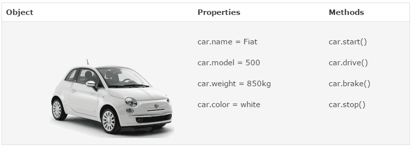
Figure 1.7: An object (https://www.w3schools.com/js/)

In R, as we will see later on, everything we work with are objects. For example, a raster—such as rainfall.tif (Appendix A)—that we import into R is actually translated to an object of a class named stars. The object has numerous properties, such as the number of raster rows and columns, the raster resolution, the Coordinate Reference System (CRS), and so on.

The following two expressions are used to import the raster rainfall.tif into the R environment (we will elaborate on that later on, in Sections 2.2 and 5.3.6):

library(stars)
r = read_stars("data/rainfall.tif")

Once imported, an object named r, belonging to the class named stars representing rasters in R, exists in the R environment (more specifically in the RAM, see Section 1.1.2). For example, printing the object displays some of its properties and their specific values. For example, we can see that the raster resolution (delta) is 1000 (meters):

r
## stars object with 2 dimensions and 1 attribute
## attribute(s):
##                   Min.  1st Qu.   Median     Mean  3rd Qu.     Max.  NA's
## rainfall.tif  200.0037 371.8833 499.5131 483.4693 587.2853 902.9678 20916
## dimension(s):
##   from  to  offset delta                refsys point x/y
## x    1 154  615965  1000 WGS 84 / UTM zone 36N FALSE [x]
## y    1 240 3691819 -1000 WGS 84 / UTM zone 36N FALSE [y]

You don’t need to worry about the meaning of the different properties in the above printout yet. For now, this is just a demonstration of what it looks like to import data into the R environment, and print some of the properties of the resulting object. We are going to return to the specific details of this operation, and the meaning of the printout components, later on when we learn about working with rasters in R (Sections 5.3.8.1–5.3.8.3, and 6.3).

1.1.5 Inheritance

One of the implications of object-oriented programming is inheritance. Inheritance makes it possible for one class to “extend” another class, by adding new properties and/or new methods. Using our car example (Figure 1.7):

• A “taxi” is an extension of the “car” class, inheriting all of its properties and methods.
• In addition to the inherited properties, a “taxi” has new properties (taxi company name) and new methods (switching the taximeter on and off).

In R, the idea of inheritance is realized in several ways. For example, every complex object (such as a raster) is actually a collection of smaller components (the properties). Looking at the structure of the raster object r (using the str function, see Section 4.1.4.2) reveals that it is, in fact, a collection of many small objects belonging to simpler classes, each holding a piece of information. For example, the raster values are stored in a numeric matrix (class matrix, see 5.1), of size \(153\times240\), as shown on the 3^rd line in the following printout. The resolution property (named delta) is stored as a numeric vector (class numeric, see Section 2.3) of length 1 (i.e., containing a single value, 1000), as shown on the 9^th line of the printout.

str(r)
## List of 1
##  $ rainfall.tif: num [1:154, 1:240] NA NA NA NA NA NA NA NA NA NA ...
##  - attr(*, "dimensions")=List of 2
##   ..$ x:List of 7
##   .. ..$ from  : num 1
##   .. ..$ to    : num 154
##   .. ..$ offset: num 615965
##   .. ..$ delta : num 1000
##   .. ..$ refsys:List of 2
##   .. .. ..$ input: chr "WGS 84 / UTM zone 36N"
##   .. .. ..$ wkt  : chr "PROJCRS[\"WGS 84 / UTM zone 36N\",\n    BASEGEOGCRS[\"WGS 84\",\n        ENSEMBLE[\"World Geodetic System 1984 "| __truncated__
##   .. .. ..- attr(*, "class")= chr "crs"
##   .. ..$ point : logi FALSE
##   .. ..$ values: NULL
##   .. ..- attr(*, "class")= chr "dimension"
##   ..$ y:List of 7
##   .. ..$ from  : num 1
##   .. ..$ to    : num 240
##   .. ..$ offset: num 3691819
##   .. ..$ delta : num -1000
##   .. ..$ refsys:List of 2
##   .. .. ..$ input: chr "WGS 84 / UTM zone 36N"
##   .. .. ..$ wkt  : chr "PROJCRS[\"WGS 84 / UTM zone 36N\",\n    BASEGEOGCRS[\"WGS 84\",\n        ENSEMBLE[\"World Geodetic System 1984 "| __truncated__
##   .. .. ..- attr(*, "class")= chr "crs"
##   .. ..$ point : logi FALSE
##   .. ..$ values: NULL
##   .. ..- attr(*, "class")= chr "dimension"
##   ..- attr(*, "raster")=List of 4
##   .. ..$ affine     : num [1:2] 0 0
##   .. ..$ dimensions : chr [1:2] "x" "y"
##   .. ..$ curvilinear: logi FALSE
##   .. ..$ blocksizes : int [1, 1:2] 154 13
##   .. .. ..- attr(*, "dimnames")=List of 2
##   .. .. .. ..$ : NULL
##   .. .. .. ..$ : chr [1:2] "x" "y"
##   .. ..- attr(*, "class")= chr "stars_raster"
##   ..- attr(*, "class")= chr "dimensions"
##  - attr(*, "class")= chr "stars"

The benefit of inheritance is that the programmer does not need to write every class from scratch. Instead, new classes can be built on top of existing ones, while re-using their properties and methods.

1.2 Starting R

Now that we covered some central theoretical concepts related to programming, we are staring the practical part—writing R code to work with spatial data. In this chapter, we will become familiar with the R environment, its basic operators and syntax rules.

To use R, we first need to install it. R can be downloaded from the R-project website. The current version at the time of writing (March 2023) is R 4.2.3. Once R is installed, we can open the default interface (RGui) with Start → All Programs → R → R x64 4.2.2 (Figure 1.8).

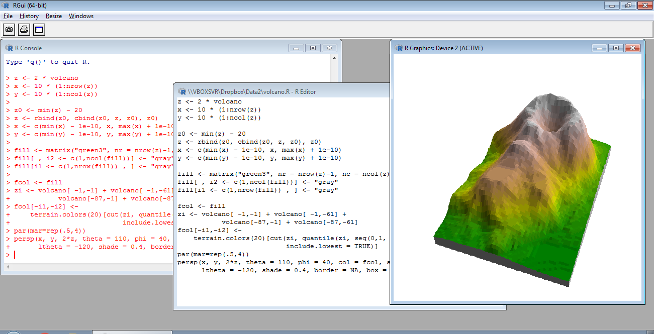
Figure 1.8: RGui

We will be working with R through a more advanced interface than the default one, called RStudio. It can be downloaded from the Posit company website. The current version, as of March 2023, is RStudio 2022.12.0-353. Once both R and RStudio are installed, we can open RStudio with Start → All Programs → RStudio → RStudio (Figure 1.9).

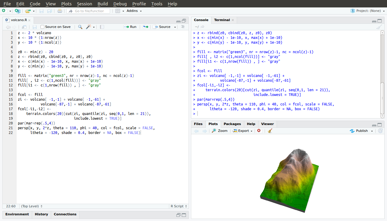
Figure 1.9: RStudio

In this Chapter, we will only work with the console, i.e., the command line. In the following lessons we will also work with other RStudio panels.

Locate the console in the RStudio interface, in the tab named “Console” (Figure 1.10).

Figure 1.10: RStudio console

Before you begin working with RStudio, it is recommended that you go to Tools→Global Options…, and then:

• Leave the Restore .RData into workspace as startup unchecked
• Set Save workspace to .RData on exit to Never

This will prevent RStudio from saving your environment when you quit, or restoring it. Instead, we will try to keep our scripts self-contained, and independent of any previous sessions, which is the recommended approach greatest reproducibility.

1.3 Basic R expressions

1.3.1 Console input and output

The simplest way to interact with the R environment is typing an expression into the R console, pressing Enter to execute it. For example, let’s type the expression 1+3+5+7:

1 + 3 + 5 + 7
## [1] 16

After we press Enter, the expression 1+3+5+7 is sent to the processor. The returned value, 16, is then printed in the console. Note that the value 16 is not kept in in the RAM or Mass Storage, just printed on screen (Figure 1.11). We will talk about what the [1] part means later on (Section 2.3.8), you can ignore it for now.

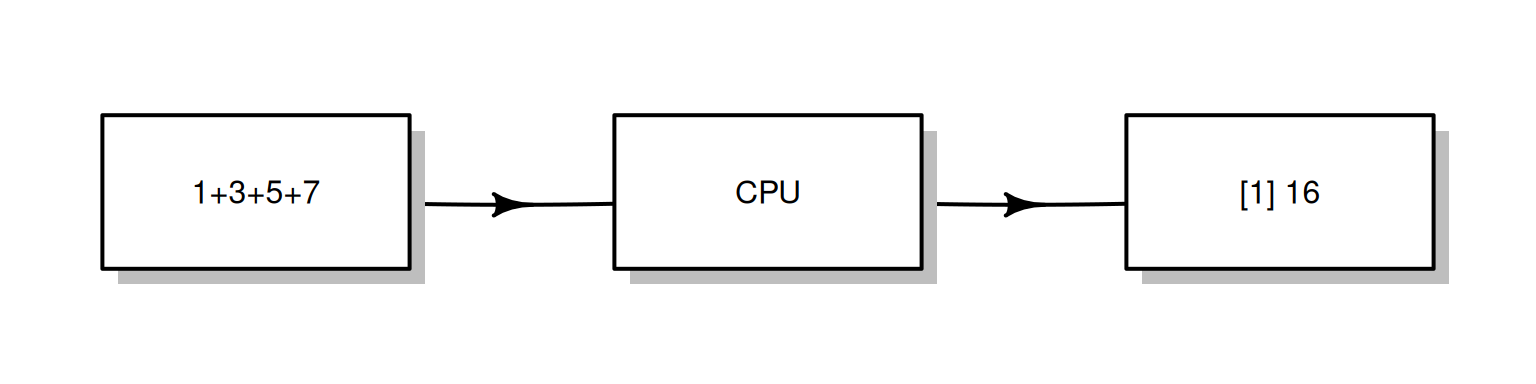
Figure 1.11: Execution of a simple expression in R

Note that, in the book, the outputs are marked with preceding two hash symbols (##), while the inputs start at the beginning of a line⁹. In RStudio, the input and output are displayed with different colors, without hash symbols (Figure 1.12).

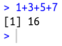
Figure 1.12: RStudio console input and output

We can type a number, the number itself is returned:

600
## [1] 600

We can type text inside single ' or double " quotes:

"Hello"
## [1] "Hello"

The last two expressions are examples of constant values, numeric or character. These are the simplest type of expressions in R.

1.3.2 Arithmetic operators

Through interactive use of the command line, we can experiment with basic operators in R. For example, R includes the standard arithmetic operators (Table 1.1).

Table 1.1: Arithmetic operators

Operator	Meaning
+	Addition
-	Subtraction
*	Multiplication
/	Division
^	Exponent

Here are some examples of expressions that use the arithmetic operators:

5 + 3
## [1] 8

4 - 5
## [1] -1

1 * 10
## [1] 10

1 / 10
## [1] 0.1

10 ^ 2
## [1] 100

We can use the up ↑ and down ↓ keys to scroll through the executed expressions history. Try to execute several different expressions, then scroll up until you reach one of the previous expressions and re-execute it by pressing Enter. Scrolling through expression history is convenient for going back to previously exceuted code, without re-typing it, possibly making modifications before excecuting it once again.

Note that very large or very small numbers are formatted in exponential notation:

1 / 1000000 # 1*10^-6
## [1] 1e-06

7 * 100000  # 7*10^5
## [1] 7e+05

Infinity is treated as a special numeric value, Inf or -Inf:

1 / 0
## [1] Inf

-1 / 0
## [1] -Inf

Inf + 1
## [1] Inf

-1 * Inf
## [1] -Inf

We can control operator precedence with brackets, just like in math:

1 + 2 * 3
## [1] 7

(1 + 2) * 3
## [1] 9

It is recommended to use brackets for clarity, even where not strictly required.

1.3.3 Spaces and comments

The interpreter ignores everything to the right of the number symbol #:

1 * 2 # * 3
## [1] 2

The # symbol is therefore used for code comments:

# Multiplication example
5 * 5
## [1] 25

Why do you think the code outputs are marked by ## in the code sections (such as ## [1] 25 in the above code section)?

The interpreter ignores spaces, so the following expressions are treated exactly the same way:

1 + 1
## [1] 2

1+1
## [1] 2

1+           1
## [1] 2

We can type Enter in the middle of an expression and keep typing on the next line. The interpreter displays the + symbol, which means that the expression is incomplete (Figure 1.13):

5 * 
2
## [1] 10

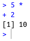
Figure 1.13: Incomplete expression

We can exit from the “completion” state, or from an ongoing computation, any time, by pressing Esc.

Clearing the console can be done with Ctrl+L.

1.3.4 Conditional operators

Conditions are expressions that use conditional operators and have a yes/no result, i.e., the condition can be either true or false. The result of a condition is a logical value, TRUE or FALSE:

• TRUE means the expression is true
• FALSE means the expression is false
• (NA means it is unknown)

The conditional operators in R are listed in Table 1.2.

Table 1.2: Conditional operators

Operator	Meaning
==	Equal
>	Greater than
>=	Greater than or equal
<	Less than
<=	Less than or equal
!=	Not equal
&	And
|	Or
!	Not

For example, we can use conditional operators to compare numeric values:

1 < 2
## [1] TRUE

1 > 2
## [1] FALSE

2 > 2
## [1] FALSE

2 >= 2
## [1] TRUE

2 != 2
## [1] FALSE

“Equal” (==) and “not equal” (!=) are opposites of each other, since a pair of values can be either equal or not:

1 == 1
## [1] TRUE
1 != 1
## [1] FALSE

1 == 2
## [1] FALSE
1 != 2
## [1] TRUE

The “and” (&) and “or” (|) operators are used to create more complex conditions. “And” (&) returns TRUE when both sides are TRUE:

(1 < 10) & (10 < 100)
## [1] TRUE

(1 < 10) & (10 > 100)
## [1] FALSE

“Or” (|) returns TRUE when at least one of the sides is TRUE:

(1 < 10) | (10 < 100)
## [1] TRUE

(1 < 10) | (10 > 100)
## [1] TRUE

The last conditional operator is “not” (!), which reverses TRUE to FALSE and FALSE to TRUE:

1 == 1
## [1] TRUE
!(1 == 1)
## [1] FALSE

(1 == 1) & (2 == 2)
## [1] TRUE
(1 == 1) & !(2 == 2)
## [1] FALSE

Run the following expression and explain their result:

FALSE == FALSE

!(TRUE == TRUE)

!(!(1 == 1))

1.3.5 Special values

R has several special values, as listed in Table 1.3.

Table 1.3: Special values in R

Value	Meaning
Inf	Infinity
NA	Not Available
NaN	Not a Number
NULL	Empty object

We already met Inf, and have shown how it can be the result of particular arithmetic operations such as division by zero (Section 1.3.2):

1 / 0
## [1] Inf

NA (“Not Available”) specifies an unknown, or missing, value. Later on, we are going to encounter several situations where NA values can arise. For example, empty cells in a table imported into R, such as from a CSV file (Section 4.4), are encoded in R as NA values.

NA values can participate in any arithmetic or logical operation. For example:

NA + 3
## [1] NA

Why do you think the result of the above expression is NA?

What do you think will be the result of the expression NA == NA?

NaN (“Not a Number”) is less relevant for the material of this book, but it is important to be familiar with it. Most commonly, NaN values arise from arithmetic operations where the result is undefined:

0 / 0
## [1] NaN

For most practical purposes, NaN values behave exactly the same way as NA values.

Finally, the value of NULL specifies an empty object:

NULL
## NULL

NULL has some uses which we will discuss later on (Section 4.2.3).

1.3.6 Functions

In math, a function (Figure 1.14) is a relation that associates each element x of a set X, to a single element y of another set Y. For example, the function \(y=2x\) is a mathematical function that associates any number \(x\) with the number \(2x\).

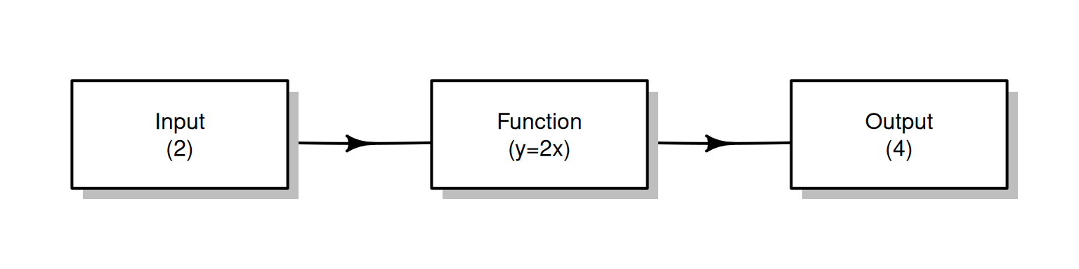
Figure 1.14: A function

The concept of functions in programming is similar. A function is a code piece that “knows” how to do a certain task. Executing the function is known as a function call. The function accepts zero or more objects as input (e.g., 2) and returns a single object as output (e.g., 4). In addition to the returned value, the function may perform other task(s), known as side effects (for example: writing information to a file, or displaying graphical output).

The number and type of inputs the function needs are determined in the function definition; these are known as the function parameters (e.g., a single number). The objects the function received in practice, as part of a particular function call, are known as arguments (e.g., 2).

A function is basically a set of pre-defined instructions. There are thousands of built-in functions in R. Later on, we will learn to define our own functions (Section 3.3).

A function call is composed of the function name, followed by the arguments inside brackets () and separated by commas ,. For example, the sqrt function calculates the square root of its input. The following expression calls the sqrt function, with the argument 4:

sqrt(4)
## [1] 2

Here, the sqrt function received a single argument, 4. It returned the square root, 2.

As a side note, it is interesting to mention that everything we do in R in fact involves functions¹⁰. Even arithmetic operators are functions, just written in a special way. The arithmetic operators can be executed in the “ordinary” function syntax, revealing they are indeed functions, as follows:

`+`(5, 5)
## [1] 10

1.3.7 Error messages

Consider the following three different expressions:

sqrt(16)
## [1] 4

sqrt("16")
## Error in sqrt("16"): non-numeric argument to mathematical function

sqrt(a)
## Error in eval(expr, envir, enclos): object 'a' not found

In last two expressions we got error messages, because the expressions were illegal, i.e., not in agreement with the syntax rules of R. The first error occurred because we tried to run a mathematical operation sqrt on a text value "a". The second error occurred because we tried to use a non-existing object a. Any text without quotes is treated as a name of an object, i.e., a label for an actual object stored in RAM. Since we don’t have an object named a we got an error.

1.3.8 Pre-loaded objects

When starting R, a default set of objects is loaded into the RAM, such as TRUE, FALSE, sqrt and pi. For example, type pi and see what happens:

pi
## [1] 3.141593

1.3.9 Decimal places

Is the value of \(\pi\) stored in memory really equal to the value we see on screen (3.141593)? Executing the following condition reveals that the answer is no:

pi == 3.141593
## [1] FALSE

If not, what is the difference?

pi - 3.141593
## [1] -3.464102e-07

The reason for the discrepancy is that, by default, R prints only the first 7 digits:

options()$digits
## [1] 7

When working with R we should keep in mind that the printed value and object contents are not always identical, because the printed output may hide certain piecies of information to make it more concise and convenient for the user.

The number of digits to print can be changed with an expression such as options(digits=22). Try running the latter expression, then print the value of pi once again.

1.3.10 Case-sensitivity

R is case-sensitive, it distinguishes between lower-case and upper-case letters. For example, TRUE is a logical value, but True and true are undefined:

TRUE
## [1] TRUE

True
## Error in eval(expr, envir, enclos): object 'True' not found

true
## Error in eval(expr, envir, enclos): object 'true' not found

1.3.11 Classes

R is an object-oriented language (Section 1.1.4), where each object belongs to a class. The class functions accepts an object and returns the class name:

class(TRUE)
## [1] "logical"

class(1)
## [1] "numeric"

class(pi)
## [1] "numeric"

class("a")
## [1] "character"

class(sqrt)
## [1] "function"

Explain the returned value of the following expressions.

class(1 < 2)
## [1] "logical"

class("logical")
## [1] "character"

class(1) == class(2)
## [1] TRUE

class(class)
## [1] "function"

class(class(sqrt))
## [1] "character"

class(class(1))
## [1] "character"

1.3.12 Using help files

Every built-in object is associated with a help document, which can be accessed using the help function or the ? operator:

help(class)
?class
?TRUE
?pi

---

9. Prefixing code output with # makes the interpreter ignore it (Section 1.3.3). That way, the entire code output can be safely copied and pasted into the interpretor.↩︎

10. “To understand computations in R, two slogans are helpful: (1) Everything that exists is an object. (2) Everything that happens is a function call.” (Chambers, 2014, Statistical Science, https://arxiv.org/pdf/1409.3531.pdf)↩︎