Chapter 5 Matrices and rasters

Last updated: 2024-07-28 11:41:29

Aims

Our aims in this chapter are:

• Start working with spatial data (rasters)
• Install and use packages beyond “base R”
• Introduce the basic matrix and array data structures, and their analogous spatial data structure (class stars) for single band and multi-band rasters, respectively
• Learn to access the cell values and other properties of rasters
• Learn to read and write raster data

We will use the following R packages:

• stars
• mapview

5.1 Matrices

5.1.1 What is a matrix?

A matrix is:

• a two-dimensional (like a data.frame) collection of values
• of the same type (like a vector, and unlike a data.frame).

The number of values in all columns of a matrix is equal, and the same can be said about the rows. It is important to know how to work with matrices because it is a commonly used data structure, with many uses in data processing and analysis, including spatial data. Many R functions accept a matrix as an argument, or return a matrix as the returned object. For example, the st_distance function returns a distance matrix between all pairs of features in two vector layers (Section 8.3.2.3). Matrices are also used for data storage in more complex data structures, e.g., to store single-band raster values in stars raster objects (as we’ll see later, in Section 5.3.8.2).

5.1.2 Creating a matrix

A matrix can be created with the matrix function. The matrix function accepts the following arguments:

• data—A vector of the values to fill into the matrix
• nrow—The number of rows
• ncol—The number of columns
• byrow—Whether the matrix is filled by column (FALSE, the default) or by row (TRUE)

For example:

x = matrix(1:6, nrow = 2, ncol = 3)
x
##      [,1] [,2] [,3]
## [1,]    1    3    5
## [2,]    2    4    6

Note that the class of matrix objects is a vector of length two, with the values 'matrix' and 'array':

class(x)
## [1] "matrix" "array"

This implies the fact that the matrix class inherits (Section 1.1.5) from the more general array class (Section 5.2).

The nrow and ncol parameters determine the number of rows and number of columns, respectively. When only one of them is specified, the other is automatically determined based on the length of the data vector:

matrix(1:6, nrow = 2)
##      [,1] [,2] [,3]
## [1,]    1    3    5
## [2,]    2    4    6

matrix(1:6, ncol = 2)
##      [,1] [,2]
## [1,]    1    4
## [2,]    2    5
## [3,]    3    6

What do you think will happen when we try to create a matrix with less, or more, data values than matrix size nrow*ncol? Run the following expressions to find out.

matrix(12:1, ncol = 4, nrow = 2)
matrix(12:1, ncol = 4, nrow = 4)

Create a \(3\times3\) matrix where all values are \(1/9\).

Finally, the byrow parameter determines the direction of filling the matrix with data values. In both cases the filling starts from the top-left corner (i.e., row 1, column 1), however with byrow=FALSE the matrix is filled one column at a time (the default), while with byrow=TRUE the matrix is filled one row at a time. For example:

matrix(1:12, nrow = 3)                ## the default (byrow=FALSE)
##      [,1] [,2] [,3] [,4]
## [1,]    1    4    7   10
## [2,]    2    5    8   11
## [3,]    3    6    9   12

matrix(1:12, nrow = 3, byrow = TRUE)  ## byrow=TRUE
##      [,1] [,2] [,3] [,4]
## [1,]    1    2    3    4
## [2,]    5    6    7    8
## [3,]    9   10   11   12

5.1.3 matrix properties

5.1.3.1 Dimensions

To demonstrate several functions for working with matrices, let’s define a matrix named x as shown above (Section 5.1.2):

x = matrix(1:6, nrow = 2)
x
##      [,1] [,2] [,3]
## [1,]    1    3    5
## [2,]    2    4    6

The length function returns the number of values in a matrix:

length(x)
## [1] 6

Just like with a data.frame (Section 4.1.4.1), the nrow and ncol functions return the number of rows and columns in a matrix, respectively:

nrow(x)
## [1] 2

ncol(x)
## [1] 3

Also like with a data.frame, the dim function gives both dimensions of the matrix as a vector of length 2, i.e., number of rows and columns, respectively:

dim(x)
## [1] 2 3

For example, R has a built-in dataset named volcano, which is a matrix of surface elevation. The sample script volcano.R, used in Section 2.1.3 to demontrate working with R code files, creates a 3D image of elevation based on that matrix (Figure 2.2).

Find out what are the number of elements, rows and columns in the built-in matrix named volcano.

5.1.3.2 Row and column names

Like a data.frame (Section 4.1.4.2), matrix objects also have row and column names which can be accessed or modified using the rownames and colnames functions, respectively. Unlike data.frame row and column names, which are mandatory, matrix row and column names are optional. For example, matrices created with matrix as shown above (Section 5.1.2) initially do not have row and column names:

rownames(x)
## NULL

colnames(x)
## NULL

The matrix row and column names can be initialized, modified, or removed, by assignment to the rownames and colnames properties:

rownames(x) = c('a', 'b')
colnames(x) = c('var1', 'var2', 'var3')
x
##   var1 var2 var3
## a    1    3    5
## b    2    4    6

rownames(x) = NULL
colnames(x) = NULL
x
##      [,1] [,2] [,3]
## [1,]    1    3    5
## [2,]    2    4    6

5.1.4 matrix conversions

5.1.4.1 matrix → vector

The as.vector function converts a matrix to a vector:

x = matrix(1:6, ncol = 3, byrow = TRUE)
x
##      [,1] [,2] [,3]
## [1,]    1    2    3
## [2,]    4    5    6

as.vector(x)
## [1] 1 4 2 5 3 6

Note that the matrix values are always arranged by column in the resulting vector!

Does the volcano matrix contain any NA values? How can we check?

5.1.4.2 matrix → data.frame

The as.data.frame function converts a matrix to a data.frame:

as.data.frame(x)
##   V1 V2 V3
## 1  1  2  3
## 2  4  5  6

Note that row and column names are automatically generated (if they do not exist) as part of the conversion, since they are mandatory in a data.frame (Section 5.1.3.2).

5.1.5 Transposing a matrix

The t function transposes a matrix. In other words, the matrix rows and columns are “switched”—rows become columns, and columns become rows:

x = matrix(1:6, ncol = 3)
x
##      [,1] [,2] [,3]
## [1,]    1    3    5
## [2,]    2    4    6

t(x)
##      [,1] [,2]
## [1,]    1    2
## [2,]    3    4
## [3,]    5    6

What will be the result of t(t(x))?

5.1.6 Image with contours

Using the image and contour functions we can graphically display matrix values in the form of a heatmap—where values are encoded to colors—and a contour layer, respectively.

The color scale in image can be set with col. R has several built-in color scale functions—such as terrain.colors and heat.colors—that return a specified number of color codes from the given color scale. The hcl.colors function offers a wider range of color scales, including many scales useful for mapping, such as the well-known ColorBrewer scales. The hcl.colors function requires the number of colors and the name of the color scale. For example, the following expression returns 11 colors from the 'Spectral' color scale:

hcl.colors(11, 'Spectral')
##  [1] "#A71B4B" "#D44D35" "#ED820A" "#F7B347" "#FCDE85" "#FEFDBE" "#BAEEAE"
##  [8] "#61D4AF" "#00B1B5" "#0084B3" "#584B9F"

The x/y aspect ratio, in either image or contour, can be set with asp.

Finally, add=TRUE can be used so that the contour layer is added on top of an existing plot, such as the one created with image, rather than initiated in a new plot.

Combining all of the above, the following expressions display a contour layer on top of a colored image of the volcano matrix. The resulting image is shown in Figure 5.1.

image(volcano, col = terrain.colors(30), asp = ncol(volcano)/nrow(volcano))
contour(volcano, add = TRUE)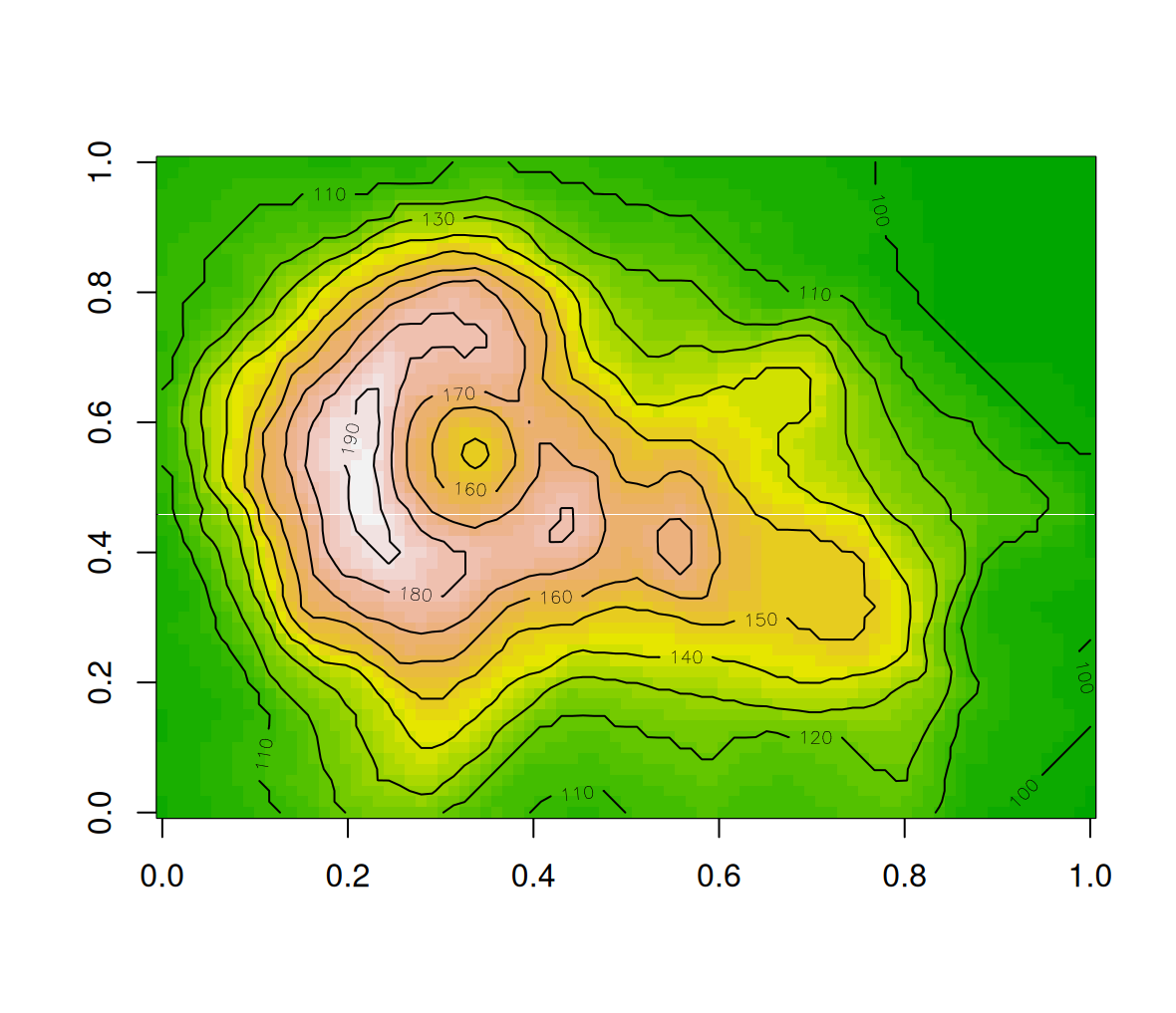

Figure 5.1: Volcano image with contours

Try replacing terrain.colors(30) with heat.colors(30), or with hcl.colors(11,'Spectral'), to see an image of the volcano matrix with other color scales. You can run hcl.pals() to get a list of possible scale types passed to hcl.colors (other than 'Spectal') and try some of those too.

Note that the argument asp=ncol(volcano)/nrow(volcano) makes sure the ratio between the x and y axes is 1:1, i.e., that the image cells are square¹⁷.

Also note that image does not display a matrix in the same orientation as its printout (rows from top to bottom, etc.). Here is the solution to obtain a matrix image in the exact same orientation (Figure 5.2):

volcano1 = t(apply(volcano, 2, rev))
image(volcano1, col = terrain.colors(30), asp = ncol(volcano1)/nrow(volcano1))
contour(volcano1, add = TRUE)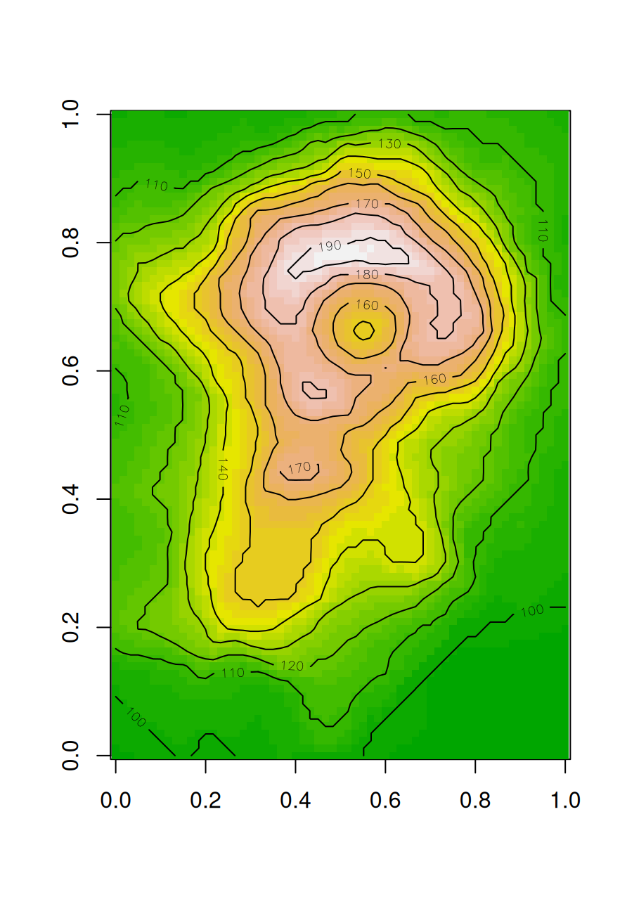

Figure 5.2: Volcano image with contours, in the same orientation as the matrix printout

5.1.7 Matrix subsetting

5.1.7.1 Individual rows and columns

Similarly to what we learned about data.frame (Section 4.1.5), matrix indices are two-dimensional. The first value refers to rows and the second value refers to columns. For example:

x
##      [,1] [,2] [,3]
## [1,]    1    3    5
## [2,]    2    4    6

x[2, 1]  # Row 2, column 1
## [1] 2

x[1, 3]  # Row 1, column 3
## [1] 5

The following examples subset the volcano matrix:

volcano[20, 40]  # Row 20, column 40
## [1] 190

volcano[81, 61]  # Row 81, column 61
## [1] 95

How can we find out the top-right corner value of volcano?

Complete rows or columns can be accessed by leaving a blank space instead of the row or column index. By default, a subset that comes from a single row or a single column is simplified to a vector:

x
##      [,1] [,2] [,3]
## [1,]    1    3    5
## [2,]    2    4    6

x[2, ]  # Row 2
## [1] 2 4 6

x[, 2]  # Column 2
## [1] 3 4

To “suppress” the simplification of individual rows/columns to a vector, we can use the drop=FALSE argument (Section 4.1.5.3):

x
##      [,1] [,2] [,3]
## [1,]    1    3    5
## [2,]    2    4    6

x[2, , drop = FALSE]  # Row 2
##      [,1] [,2] [,3]
## [1,]    2    4    6

x[, 2, drop = FALSE]  # Column 2
##      [,1]
## [1,]    3
## [2,]    4

When referring to an elevation matrix, such as volcano, any given row or column subset is actually an elevation profile. For example, the following expressions extract two elevation profiles from volcano:

r30 = volcano[30, ]  # Row 30
r70 = volcano[70, ]  # Row 70

Figure 5.3 graphically displays those profiles (Section 3.2.1):

plot(r30, type = 'o', col = 'blue', ylim = range(c(r30, r70)), ylab = 'Elevation (m)')
lines(r70, type = 'o', col = 'red')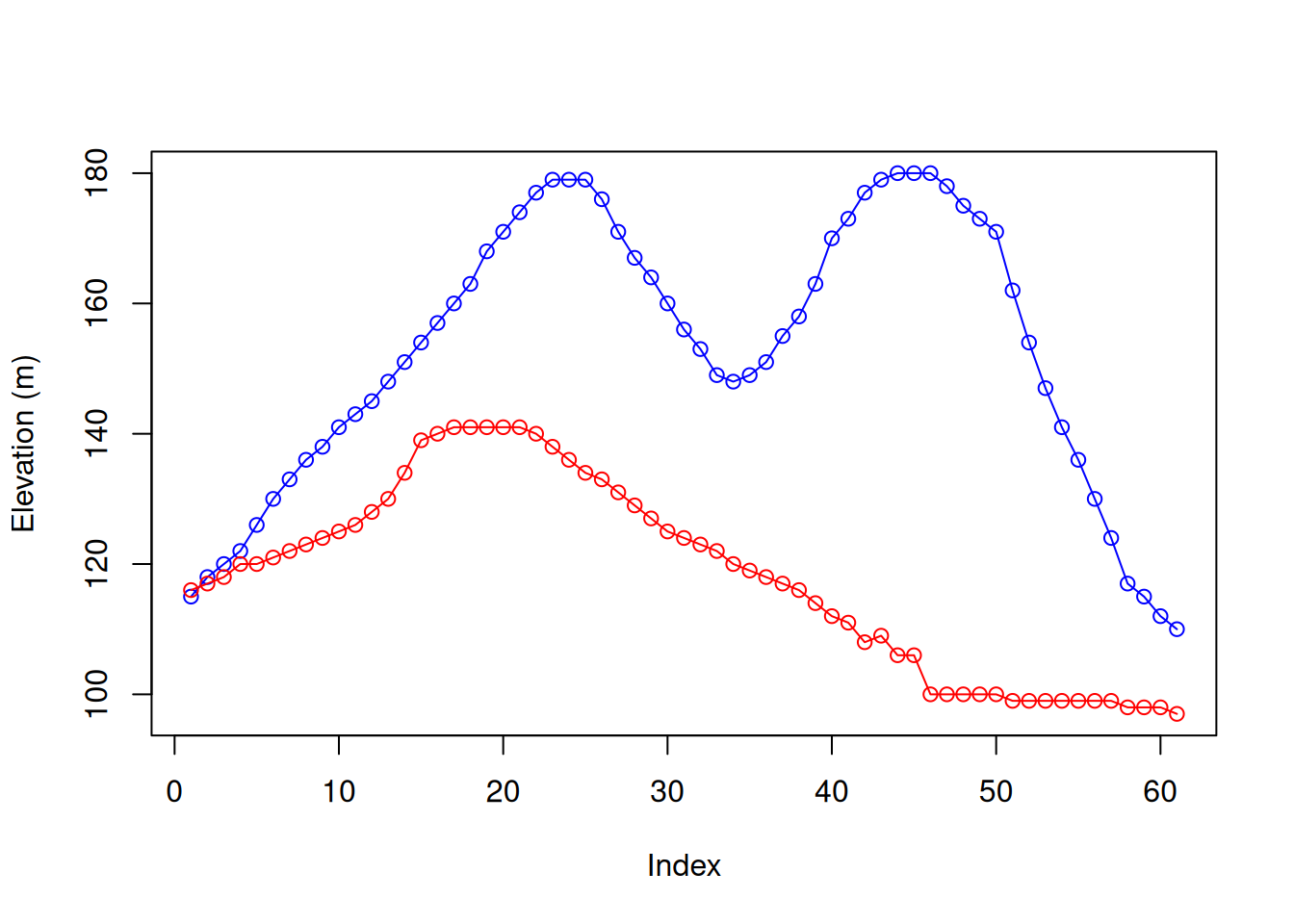

Figure 5.3: Rows 30 (blue) and 70 (red) from the volcano matrix

Figure 5.4 shows the location of the two profiles in a 3D image of volcano.

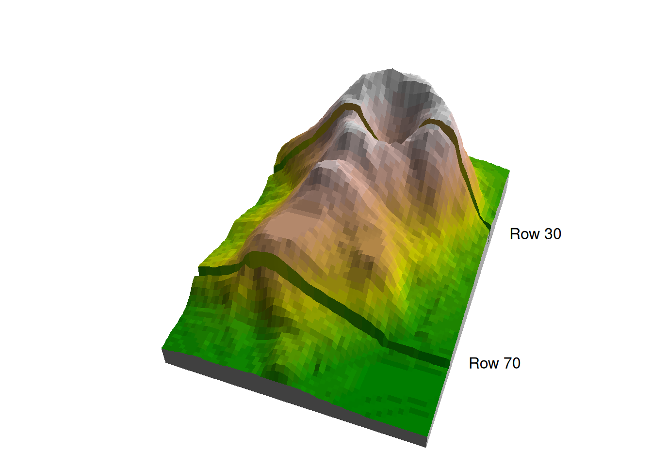
Figure 5.4: Rows 30 and 70 in the volcano matrix

5.1.7.2 Subsets with >1 row or column

We can also use vectors of length >1 when subsetting:

x
##      [,1] [,2] [,3]
## [1,]    1    3    5
## [2,]    2    4    6

x[, 1:2]
##      [,1] [,2]
## [1,]    1    3
## [2,]    2    4

x[2, c(1,3)]
## [1] 2 6

x[2, c(1,3), drop = FALSE]
##      [,1] [,2]
## [1,]    2    6

We can assign new values to subsets of a matrix:

m = matrix(NA, ncol = 3, nrow = 3)
m
##      [,1] [,2] [,3]
## [1,]   NA   NA   NA
## [2,]   NA   NA   NA
## [3,]   NA   NA   NA

m[2:3, 1:2] = 1
m
##      [,1] [,2] [,3]
## [1,]   NA   NA   NA
## [2,]    1    1   NA
## [3,]    1    1   NA

m[1:2, 2:3] = 100
m
##      [,1] [,2] [,3]
## [1,]   NA  100  100
## [2,]    1  100  100
## [3,]    1    1   NA

5.1.8 Summarizing rows and columns

How can we calculate the row or column means of a matrix? One way is to use a for loop (Section 4.2.3), as follows:

result = rep(NA, nrow(volcano))
for(i in 1:nrow(volcano)) {
  result[i] = mean(volcano[i, ])
}

The resulting vector of row means can be visualized as follows (Figure 5.5):

plot(result, type = 'b', xlab = 'Row', ylab = 'Elevation (m)')

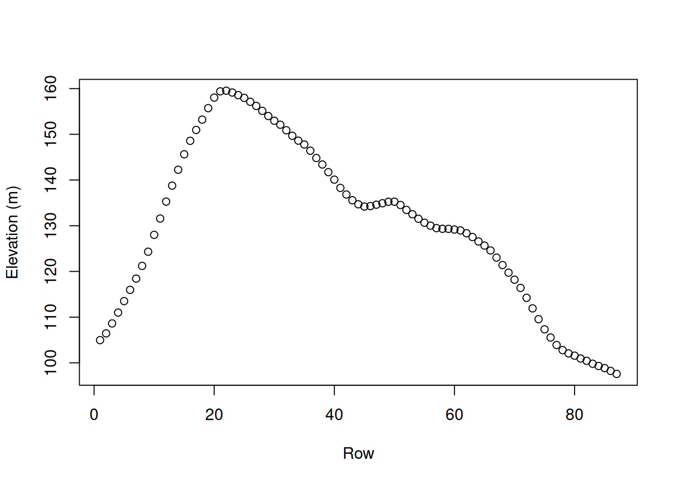
Figure 5.5: Row means of volcano

What changes do we need to make in the for loop code to calculate column means?

We can use the apply function (Section 4.5) to do the same, using much shorter code:

result = apply(volcano, 1, mean)

What changes do we need to make in the apply expression to calculate column means?

Moreover, for the special case of mean there are further shortcuts, named rowMeans and colMeans¹⁸:

result = rowMeans(volcano)

Note: in both cases we can use na.rm to determine whether NA values are included in the calculation (default is FALSE).

How can we check whether the above two expressions give exactly the same result?

5.2 Arrays

5.2.1 Creating an array

An array is a data structure that contains values of the same type and can have any number of dimensions. We may therefore consider a vector (1 dimension) and a matrix (2 dimensions) as special cases of an array. In this scope of this book, we will be dealing only with three-dimensional arrays, which—as we will see later on (Section 5.3.8.2)—are used to store multi-band raster values in stars raster objects.

An array can be created with the array function, specifying the values (data) and the required dimensions (dim). Note that creating arrays, with the array function, is very similar to the way we create matrices, with the matrix function—just more general. For example, the following expression creates an array with the values 1:24 and three dimensions—2 rows, 3 columns, and 4 “layers” (Figure 5.6):

y = array(data = 1:24, dim = c(2, 3, 4))
y
## , , 1
## 
##      [,1] [,2] [,3]
## [1,]    1    3    5
## [2,]    2    4    6
## 
## , , 2
## 
##      [,1] [,2] [,3]
## [1,]    7    9   11
## [2,]    8   10   12
## 
## , , 3
## 
##      [,1] [,2] [,3]
## [1,]   13   15   17
## [2,]   14   16   18
## 
## , , 4
## 
##      [,1] [,2] [,3]
## [1,]   19   21   23
## [2,]   20   22   24

Figure 5.6: An array with 2 rows, 3 columns and 4 “layers”. This figure is from Wickham et al. (2011).

5.2.2 Array subsetting

Subsetting an array works similarly to matrix subsetting (Section 5.1.7), only that we can have any number of indices—corresponding to the number of array dimensions—rather than two. Specifically, when subsetting a three-dimensional array we need to provide three indices. For example, here is how we can extract a particular row, column or “layer” from a three-dimensional array (Figure 5.7):

y[1, , , drop = FALSE]  # Row 1
## , , 1
## 
##      [,1] [,2] [,3]
## [1,]    1    3    5
## 
## , , 2
## 
##      [,1] [,2] [,3]
## [1,]    7    9   11
## 
## , , 3
## 
##      [,1] [,2] [,3]
## [1,]   13   15   17
## 
## , , 4
## 
##      [,1] [,2] [,3]
## [1,]   19   21   23

y[, 1, , drop = FALSE]  # Column 1
## , , 1
## 
##      [,1]
## [1,]    1
## [2,]    2
## 
## , , 2
## 
##      [,1]
## [1,]    7
## [2,]    8
## 
## , , 3
## 
##      [,1]
## [1,]   13
## [2,]   14
## 
## , , 4
## 
##      [,1]
## [1,]   19
## [2,]   20

y[, , 1, drop = FALSE]  # "Layer" 1
## , , 1
## 
##      [,1] [,2] [,3]
## [1,]    1    3    5
## [2,]    2    4    6

Figure 5.7: array subsetting: selecting one row, column or “layer”. This figure is from Wickham et al. (2011).

We can also subset two or three dimensions at a time, to get an individual row/column, row/layer, column/layer or row/column/layer combination (Figure 5.8):

y[1, 1, ]  # Row 1, column 1
## [1]  1  7 13 19

y[1, , 1]  # Row 1, "layer" 1
## [1] 1 3 5

y[, 1, 1]  # Column 1, "layer" 1
## [1] 1 2

y[1, 1, 1]  # Row 1, column 1, "layer" 1
## [1] 1

Figure 5.8: array subsetting. This figure is from Wickham et al. (2011).

5.2.3 Using apply with arrays

When using apply on a 3-dimensional array, we can apply a function:

• On one of the dimensions: rows (1), columns (2), or “layers” (3)
• On a combinations of any two dimensions: row/column combinations (c(1,2)), row/“layer” combinations (c(1,3)), or column/“layer” combinations (c(2,3))

For example:

apply(y, 1, mean)    # Row means
## [1] 12 13

apply(y, 2, mean)    # Column means
## [1] 10.5 12.5 14.5

For arrays representing spatial data, i.e., multi-band rasters, the two most useful dimension combinations are summarizing layer or pixel properties (Section 5.3). For example:

apply(y, 3, mean)    # "Layer" means
## [1]  3.5  9.5 15.5 21.5

apply(y, 1:2, mean)  # Row/Column combination ("pixel") means
##      [,1] [,2] [,3]
## [1,]   10   12   14
## [2,]   11   13   15

5.2.4 Basic data structures in R

So far, we met four out of five of the basic data structures in R (Table 5.1). It is time for a short summary. We can classify the basic data structures in R based on:

• Number of dimensions—
  • One-dimensional¹⁹
  • 2-dimensional
  • N-demensional
• Homogeneity—
  • Homogeneous (values of the same type)
  • Heterogeneous (values of different types)

Table 5.1: Five basic data structures in R

Dimensions	Homogeneous	Heterogeneous
One-dimensional	vector (numeric, character, logical, Date) (Chapter 2)	list (Chapter 11)
Two-dimensional	matrix (Chapter 5)	data.frame (Chapter 4)
N-dimensional	array (Chapter 5)

Most of the data structures in R are combinations of these basic five ones.

5.3 Rasters

5.3.1 What is a raster?

A raster (Figure 5.9) is basically a matrix or an array representing a rectangular area on the surface of the earth. To associate a matrix, or an array, with the particular area it represents, the raster has some additional spatial properties:

• Origin (\(x_{min}\), \(y_{max}\)) and resolution (\(delta_{x}\), \(delta_{y}\))
• Coordinate Reference System (CRS)

on top of the non-spatial properties that any ordinary matrix or array has:

• Values
• Dimensions (rows, columns, layers)

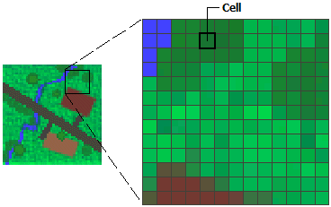
Figure 5.9: Raster cells (http://desktop.arcgis.com/en/arcmap/10.3/manage-data/raster-and-images/what-is-raster-data.htm)

Let’s now clarify the spatial property terms listed above: origin, resolution, and CRS.

The purpose of the the origin and resolution is to convey the coordinates of all raster pixels. Since the raster is regular (i.e., its rows and columns are parallel to the axes, and step size in the x and y direction is fixed), there is no need to actually store all coordinate values: just four numbers are sufficient to calculate them. Raster origin is the location of the top-left corner of the raster, i.e., the top-left corner of the top-left raster pixel (\(x_{min}\), \(y_{max}\)). Raster resolution is the step size between one pixel to the next, in the x and y directions (\(delta_{x}\), \(delta_{y}\)). Knowing the origin and resolution, the x- and y-coordinates of each pixel at (\(row\), \(col\)) can be calculated using Equations (5.1) and (5.2), respectively.

\[\begin{equation} x = x_{min} + (delta_{x} \times col) - (\frac{1}{2} \times delta_{x}) \tag{5.1} \end{equation}\]

\[\begin{equation} y = y_{max} + (delta_{y} \times row) - (\frac{1}{2} \times delta_{y}) \tag{5.2} \end{equation}\]

In plain language, to get the pixel coordinates we start from the origin, then go the specified number of steps along the axis, whereas step size is the resolution. Additionally, we subtract half of the step size, to get the coordinates of the pixel centroid, rather than the coordinates of its edge. By convention, the y-axis origin is specified as the maximum value (i.e., \(y_{max}\)), and, accordingly, the y-axis resolution is negative (we elaborate on this in Section 6.3.3).

Another commonly used raster property is the extent, the range of x- and y-axis coordinates that the raster occupies (Figure 5.10), that is, a set of four numbers: \(x_{min}\), \(y_{min}\), \(x_{max}\), \(y_{max}\). Raster extent holds the same information as the origin+resolution, and the two are interchangeable. Namely, given the origin, resolution, and the dimensions (number of rows and columns), we can always calculate the extent, and vice versa. For example, the x-axis resolution is equal to the x-axis range difference (i.e., \(x_{max}-x_{min}\)) divided by the number of columns. Therefore, in the leftmost panel in Figure 5.10, the x-axis and y-axis resolutions are both equal to \(\frac{8-0}{12}=\frac{8}{12}\approx 0.67\).

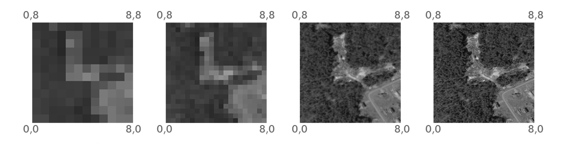
Figure 5.10: Rasters with the same extent but four different resolutions (http://datacarpentry.org/organization-geospatial/01-intro-raster-data/index.html)

As shown above, given the origin+resolution, we can determine the coordinates of all raster pixels. However, bare coordinates are just numbers. It is the Coordinate Reference System (CRS) definition that ties the coordinates to specific locations on the surface of the Earth. The CRS is the particular system that “associates” the raster coordinates (which are just pairs of x/y values) to geographic locations. For example, in the WGS84 geographic CRS, the point (0,0) (known as Null Island²⁰) is located in the Gulf of Guinea, in the Atlantic Ocean. In a different CRS, the (0,0) pair of coordinates may refer to a completely different location, or even a location supposedly beyond the surface of the Earth. Therefore, we must know the CRS to “make sense” of numeric coordinates.

5.3.2 Raster file formats

Commonly used raster file formats (Table 5.2) can be divided in two groups. “Simple” raster file formats, such as GeoTIFF, are single-band or multi-band rasters (Figure 5.11) with a geo-referenced extent, as discussed above (Section 5.3.1). “Complex” raster file formats, such as HDF, contain additional complexity, such as more than three dimensions (Figure 5.12), and/or metadata, such as band names, time stamps, units of measurement, and so on.

Table 5.2: Common raster file formats

Type	Format	File extension
“Simple”	GeoTIFF	.tif
	Erdas Imagine Image	.img
“Complex” (>3D and/or metadata)	HDF	e.g., .hdf or he5
	NetCDF	.nc

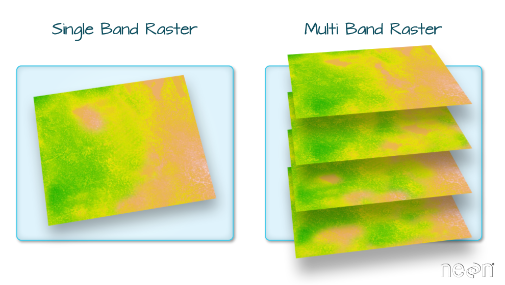
Figure 5.11: Single-band and multi-band raster (https://datacarpentry.org/organization-geospatial/)

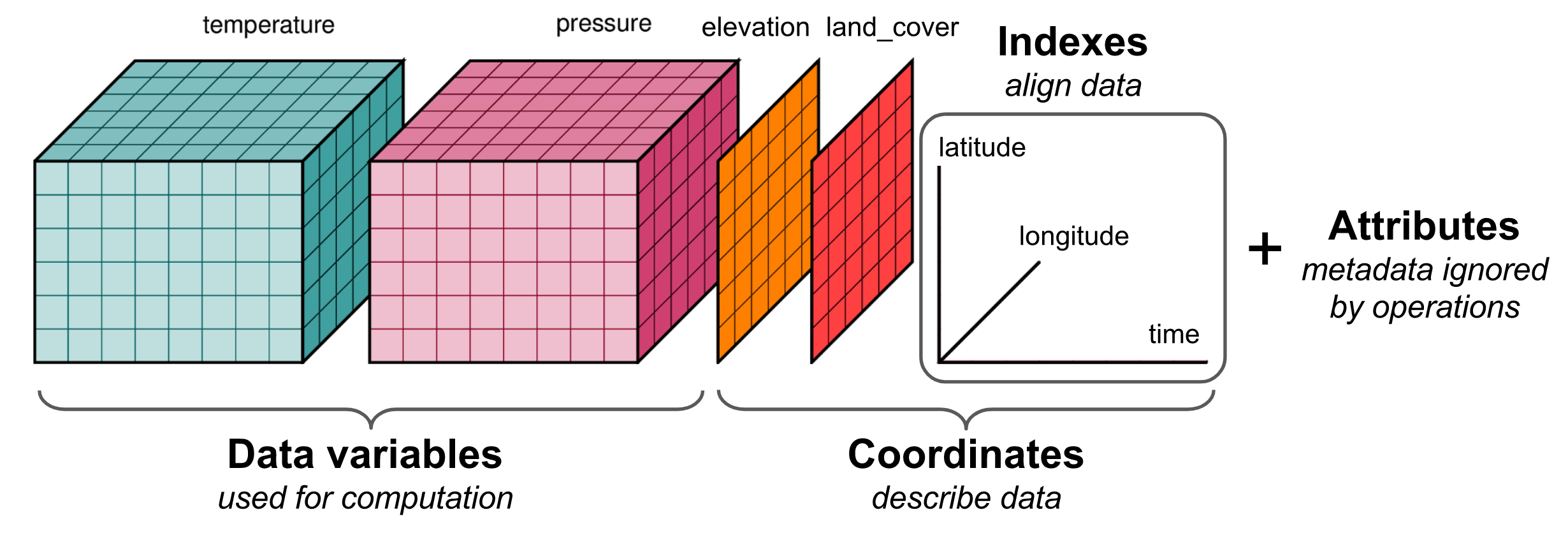
Figure 5.12: An example of an HDF file structure (http://matthewrocklin.com/blog/work/2018/02/06/hdf-in-the-cloud)

5.3.3 Using R packages

Functions for working with rasters are not included in the “base” R installation, but in external packages, such as the stars package, which we are going to learn about in a moment (Section 5.3.5). Before that, let’s say a few words about what exactly are R packages, and how to use them.

An R package is a collection of code files used to load objects—mostly functions—into memory. All object definitions in R are contained in packages. To use a particular package, we need to:

• Install the package with the install.packages function (once, for every installation of R²¹)
• Load the package using the library function (every time we start a new R session)

Installing a package with install.packages downloads the package code from a repository and stores it on our computer. Loading a package with library basically means that all of its code files are executed, loading all objects the package defined into the RAM.

Note that all function calls we used until now did not require installing or loading any package. Why is that? The answer is that several packages are installed along with R and loaded on R start-up (known as “base” packages). There are several more packages which are installed by default but not loaded on start-up (known as “recommended packages”). The number of packages in both of these groups is 29, as of May 2024 (Table 5.3).

Table 5.3: Packages included with the installaton of R as of May 2024, including “base” packages (loaded by default), and “recommended” packages (installed but not loaded default)

Package	Version	Priority
base	4.4.0	base
compiler	4.4.0	base
datasets	4.4.0	base
graphics	4.4.0	base
grDevices	4.4.0	base
grid	4.4.0	base
methods	4.4.0	base
parallel	4.4.0	base
splines	4.4.0	base
stats	4.4.0	base
stats4	4.4.0	base
tcltk	4.4.0	base
tools	4.4.0	base
utils	4.4.0	base
boot	1.3-30	recommended
class	7.3-22	recommended
cluster	2.1.6	recommended
codetools	0.2-19	recommended
foreign	0.8-86	recommended
KernSmooth	2.23-22	recommended
lattice	0.22-5	recommended
MASS	7.3-60	recommended
Matrix	1.6-5	recommended
mgcv	1.9-1	recommended
nlme	3.1-163	recommended
nnet	7.3-19	recommended
rpart	4.1.23	recommended
spatial	7.3-15	recommended
survival	3.5-8	recommended

Most of the ~20,775 official R packages (as of May 2024) are not installed by default. To use one of these packages we first need to install it on the computer. Installing a package is a one-time operation using the install.packages function. After the package is installed, each time we want to use it we need to load it using library.

In the following examples, we are going use a package called stars to work with rasters. The stars package is not installed with R, therefore we need to install it ourselves with:

install.packages('stars')

If the package is already installed, running install.packages overwrites the old installation. This is done intentionally if you you want to update the package, i.e., to install a newer version of the package.

Once the package is installed, we need to use the library function to load it into memory. Note how the package name can be passed to library (with or without quotes):

library(stars)

Other than stars, in this book we are going to use the mapview, sf, units, data.table, dplyr, gstat, and automap packages. You can now take the time and install all of them, using a series of install.packages expressions, or all of them at once with:

install.packages(c('stars','mapview','sf','units','data.table','dplyr','gstat','automap'))

5.3.4 The raster and terra packages

Before moving on to stars package, the raster and terra packages deserve to be mentioned. The raster package is a powerful and well-established (2010-) package for working with rasters in R (Table 0.1). terra (2020-) is the new and improved package by the same authors, providing very similar capabilities, only easier to use, and faster. Each of these packages contains several classes, and a very extensive collection of functions, for working with rasters in R.

The raster and terra packages have several limitations compared to stars, most notably that they are limited to three dimensions, and cannot hold raster metadata such as measurement units. Moreover, they are less well-integrated with the sf package—which is the leading package for working with vector layers in R (Chapters 7–8). On the other hand, raster and terra provide some “classical” GIS operations that are unavialble in stars, such as built-in focal filter functions (Section 9.4). Otherwise, however, there is a very large overlap between stars and raster/terra in terms of capabilities, and the choice is ultimately a matter of preference. In this book we will be working with the stars package for rasters (Section 5.3.5), which we now move on to introduce.

5.3.5 The stars package

The stars package is a relatively new (2018-) R package for working with rasters (Table 0.1). The stars package is comprehensive, flexible, and tightly integrated with the leading package for vector layers named sf, which we learn about later on (Section 7.1.4).

The stars package defines the stars class, used for representing all types of rasters, and numerous functions for working with rasters in R. A stars object is basically a list of matrices or arrays, along with metadata describing their dimensions. Don’t worry if this is not clear; we will elaborate on this shortly (Section 6.3).

Notably, the stars class is very flexible, and can represent complex rasters:

• Rasters with more than three dimensions
• Metadata (band names, units of measurement, etc.)
• Non-regular raster grids (rotated/sheared, rectilinear, or curvilinear)

In this book we are going to work with “simple” regular rasters, such as those typically stored in GeoTIFF files (Section 5.3.2). Nevertheless, it is important to be aware that stars can handle a wide variety of raster complexity which you may encounter in more specialized use cases, which are beyond the scope of this book, such as when working with climatic datasets (Figure 5.12).

5.3.6 Reading raster from file

The most common and most useful method for creating a raster object in R (and elsewhere) is reading from a file, such as a GeoTIFF file. We can use the read_stars function to read a GeoTIFF file and create a stars object in R. The first parameter (.x) is the file path to the file we want to read, or just the file name—when the file is located in the working directory.

As an example, let’s read the dem.tif raster file, which contains a coarse Digital Elevation Model (DEM) of the area around Haifa. First, we have to load the stars package:

library(stars)

Then, we can use the read_stars function to read the file into a stars object named s²²:

s = read_stars('data/dem.tif')

The file MOD13A3_2000_2019.tif is a multi-band raster with monthly Normalized Difference Vegetation Index (NDVI) values in Israel, for the period between February 2000 and June 2019 from the MODIS instrument on the Terra satellite. This is a multi-band raster with 233 bands, where each band corresponds to an average monthly NDVI image (233 months in total). Uncertain NDVI values, such as in clouded areas, were replaced with NA. Let’s try reading this file as well, to create another stars object, named r, in the R environment:

r = read_stars('data/MOD13A3_2000_2019.tif')

Two stars objects, named r and s, are now available in our R session.

5.3.7 Visualization with plot and mapview

5.3.7.1 Raster images with plot

The simplest way to visualize a stars object is to use the plot function. This produces a static image of the raster, such as the ones shown in Figures 5.13 and 5.14:

plot(s)

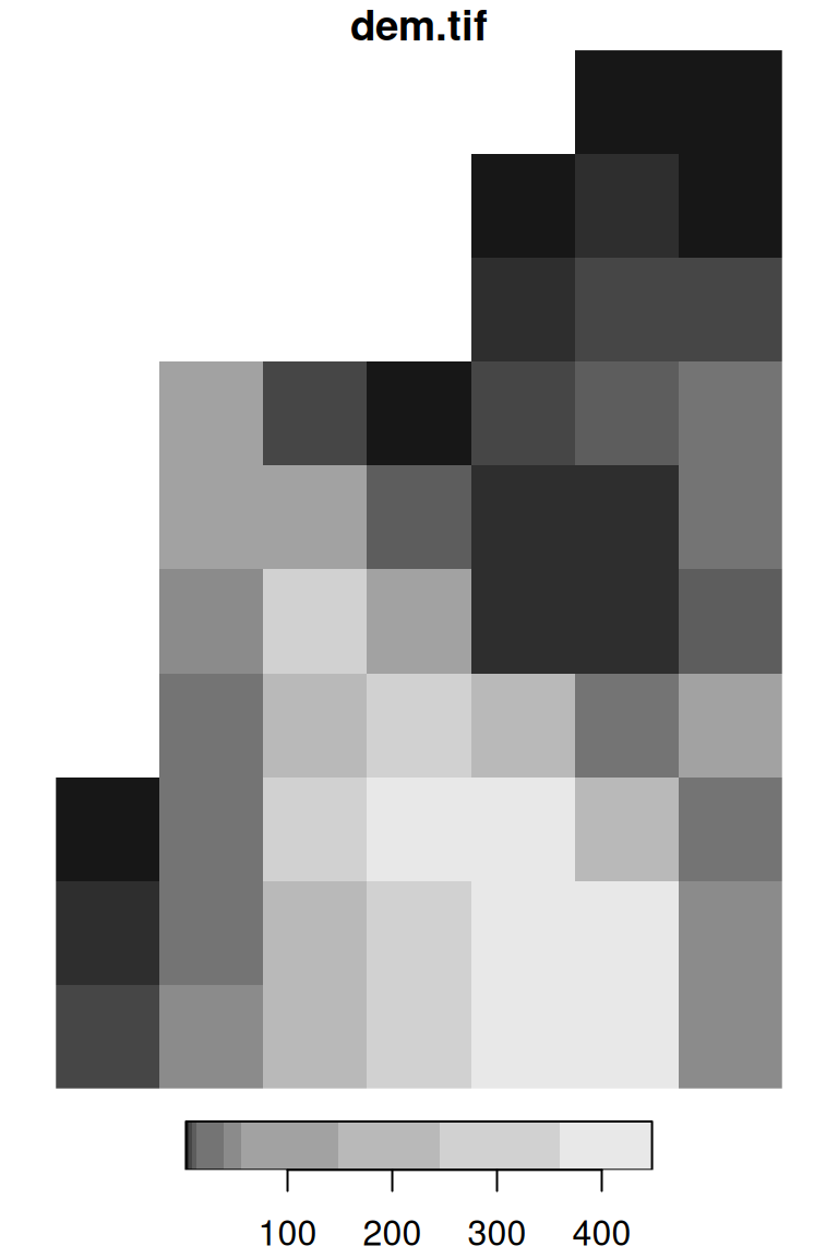
Figure 5.13: A default raster plot output: single-band raster

plot(r)
## downsample set to 2

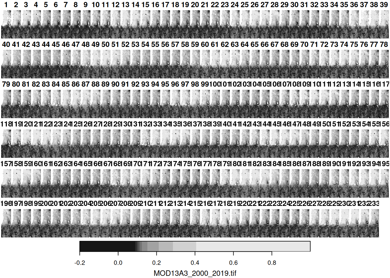
Figure 5.14: A default raster plot output: multi-band raster

Useful additional parameters when running plot on stars objects include:

• text_values—Logical, whether to display text labels (default is FALSE)
• axes—Logical, whether to display axes (default is FALSE)
• col—A vector of color codes or names

For example (Figure 5.15):

plot(s, text_values = TRUE, axes = TRUE, col = terrain.colors(10))

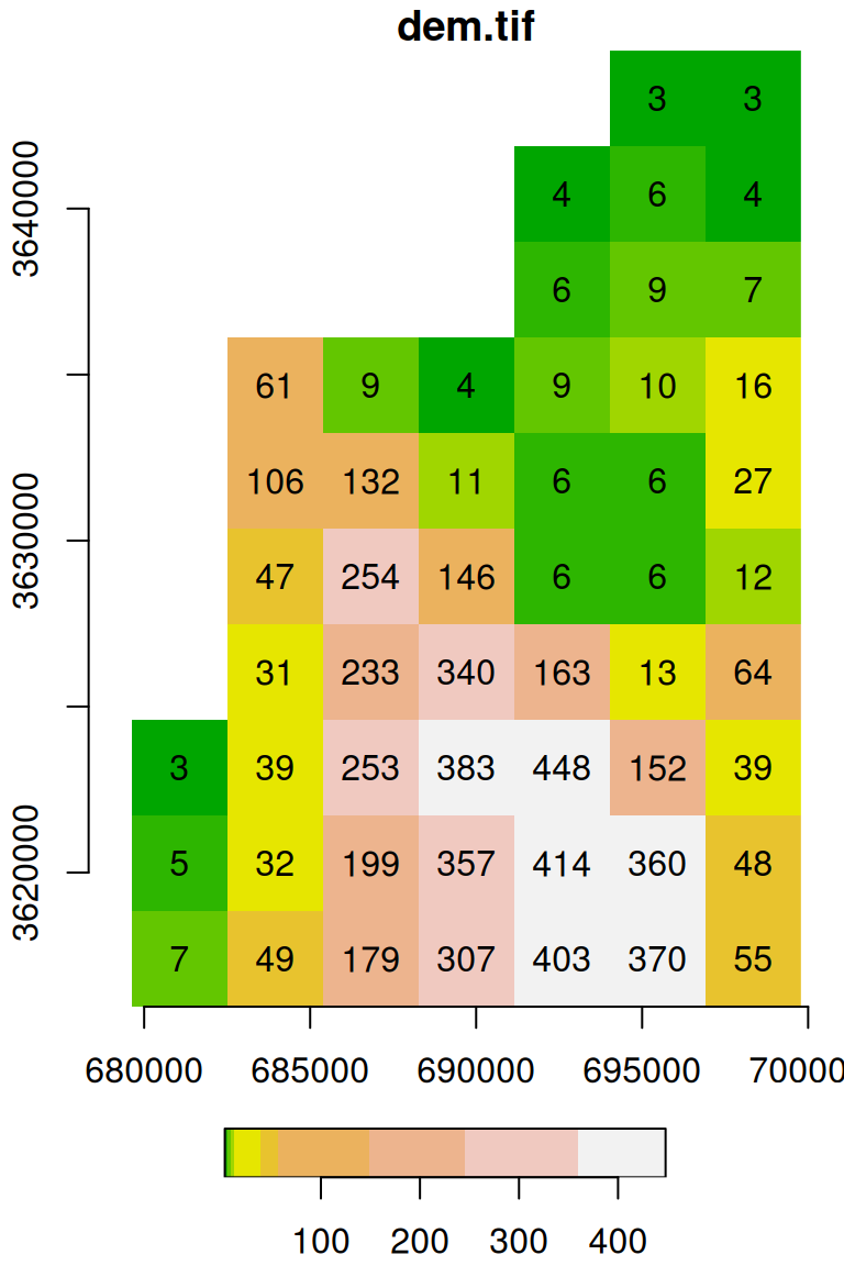
Figure 5.15: Raster plot with additional parameters text_values, axes, and col

The expression terrain.colors(10) uses one of the built-in color palette functions in R to generate a vector of length 10 with terrain color codes, as discussed above (Section 5.1.6). The default color breaks are calculated using quantiles (breaks='quantile'). We can use other break types (e.g., breaks='equal'), or pass our own vector of custom breaks (Figure 5.16):

plot(s, text_values = TRUE, col = terrain.colors(10), breaks = 'equal')
plot(s, text_values = TRUE, col = terrain.colors(3), breaks = c(0, 100, 300, 500))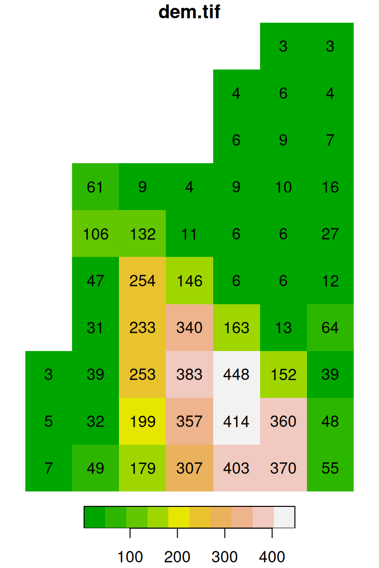

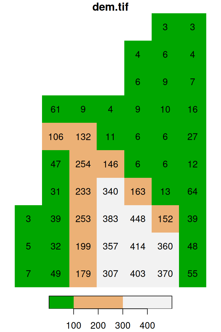
Figure 5.16: Evenly spaced color breaks using breaks='equal' (left) and manually defined breaks using breaks=c(0,100,300,500) (right)

Note that the number of colors in the second expression (e.g., 4) needs to match the number of breaks minus one (e.g., 3) (why?).

5.3.7.2 Interactive maps with mapview

The mapview function from package mapview lets us visually examine spatial objects—vector layers or rasters—in an interactive map on top of various background layers, such as OpenStreetMap, satellite images, etc. We can use the mapview function, after loading the mapview package, as follows. In this case, we are displaying the second layer of r (we learn about layer subsetting in Section 6.2.1):

library(mapview)
mapview(r[,,,2])

---

5.3.8 Raster values and properties

5.3.8.1 Class and structure

Before moving on to cover the structure and properties of stars objects (Section 5.3.8.2–5.3.8.3), let us get a sense of the way their structure is reflected in the R console through the print, class, and str commands.

The print method for raster objects gives a summary of their properties:

s
## stars object with 2 dimensions and 1 attribute
## attribute(s):
##          Min. 1st Qu. Median     Mean 3rd Qu. Max. NA's
## dem.tif     3       7     39 110.4906     179  448   17
## dimension(s):
##   from to  offset delta                       refsys point x/y
## x    1  7  679624  2880 UTM Zone 36, Northern Hem... FALSE [x]
## y    1 10 3644759 -2880 UTM Zone 36, Northern Hem... FALSE [y]

The class function returns the class name, which is stars in this case:

class(s)
## [1] "stars"

As discussed in Section 1.1.4, a class is a “template” with pre-defined properties that each object of that class has. For example, a stars object is actially a collection (namely, a list) of matrix or array objects, along with additional properties of the dimensions, such as dimension names, Coordinate Reference Systems (CRS), etc. When we read the dem.tif file with read_stars, the information regarding all of the properties was transferred from the file and into the stars “template”. Now, the stars object named s is in the RAM, filled with the specific values from dem.tif.

We can display the structure of the stars object with the specific values with str:

str(s)
## List of 1
##  $ dem.tif: num [1:7, 1:10] NA NA NA NA NA 3 3 NA NA NA ...
##  - attr(*, "dimensions")=List of 2
##   ..$ x:List of 7
##   .. ..$ from  : num 1
##   .. ..$ to    : num 7
##   .. ..$ offset: num 679624
##   .. ..$ delta : num 2880
##   .. ..$ refsys:List of 2
##   .. .. ..$ input: chr "UTM Zone 36, Northern Hemisphere"
##   .. .. ..$ wkt  : chr "PROJCRS[\"UTM Zone 36, Northern Hemisphere\",\n    BASEGEOGCRS[\"WGS 84\",\n        DATUM[\"unknown\",\n       "| __truncated__
##   .. .. ..- attr(*, "class")= chr "crs"
##   .. ..$ point : logi FALSE
##   .. ..$ values: NULL
##   .. ..- attr(*, "class")= chr "dimension"
##   ..$ y:List of 7
##   .. ..$ from  : num 1
##   .. ..$ to    : num 10
##   .. ..$ offset: num 3644759
##   .. ..$ delta : num -2880
##   .. ..$ refsys:List of 2
##   .. .. ..$ input: chr "UTM Zone 36, Northern Hemisphere"
##   .. .. ..$ wkt  : chr "PROJCRS[\"UTM Zone 36, Northern Hemisphere\",\n    BASEGEOGCRS[\"WGS 84\",\n        DATUM[\"unknown\",\n       "| __truncated__
##   .. .. ..- attr(*, "class")= chr "crs"
##   .. ..$ point : logi FALSE
##   .. ..$ values: NULL
##   .. ..- attr(*, "class")= chr "dimension"
##   ..- attr(*, "raster")=List of 4
##   .. ..$ affine     : num [1:2] 0 0
##   .. ..$ dimensions : chr [1:2] "x" "y"
##   .. ..$ curvilinear: logi FALSE
##   .. ..$ blocksizes : int [1, 1:2] 7 10
##   .. .. ..- attr(*, "dimnames")=List of 2
##   .. .. .. ..$ : NULL
##   .. .. .. ..$ : chr [1:2] "x" "y"
##   .. ..- attr(*, "class")= chr "stars_raster"
##   ..- attr(*, "class")= chr "dimensions"
##  - attr(*, "class")= chr "stars"

The 1^st line in the str printout, tells us that the s raster object is a list of length 1, namely that the raster has one attribute. The 2^nd line in the str printout specifies the name and contents of the first (and only) item in the list, namely its type, dimensions, and a sample of the first few values. In this case, the list item is named 'dem.tif', and it is a matrix with 7 rows and 10 columns. We elaborate on raster values and methods to access them in Sections 5.3.8.2, 5.3.8.4, and 6.2. The remaining lines in the str printout comprise the 'dimensions' component of the raster object, which contains the spatial properties of the raster. We elaborate on the 'dimensions' component of rasters in Sections 5.3.8.3 and 6.3.

Recall that “simple” rasters (Section 5.3.2), such as the ones we are working with in this book, always contain just one attribute.

5.3.8.2 Raster attributes and values

stars objects are collections of matrices or arrays. Each matrix or array is known as an attribute and is associated with a name. A GeoTIFF file, being a simple raster format (Section 5.3.2), can contain just one attribute. Attribute names are not specified as part of a GeoTIFF file, and therefore automatically given default values based on the file name. We can get the attribute name(s) using the names function:

names(s)
## [1] "dem.tif"

names(r)
## [1] "MOD13A3_2000_2019.tif"

We can change the attribute names through assignment. For example, it makes sense to name the attribute after the physical property or measurement it represents:

names(s) = 'elevation'
names(s)
## [1] "elevation"

names(r) = 'NDVI'
names(r)
## [1] "NDVI"

Accessing an attrubute, by name or by numeric index, returns the matrix (if single-band raster) or array (if multi-band raster) object with the values of that attribute. Accessing attributes uses the list access methods (Section 11.1.2), namely:

• list$name
• list[[index]]
• list[['name']]

where list is the list object, name is the element name, and index is the element’s numeric index.

For example, in the following expressions we access the (only) attribute of the s raster by name:

s$elevation
##      [,1] [,2] [,3] [,4] [,5] [,6] [,7] [,8] [,9] [,10]
## [1,]   NA   NA   NA   NA   NA   NA   NA    3    5     7
## [2,]   NA   NA   NA   61  106   47   31   39   32    49
## [3,]   NA   NA   NA    9  132  254  233  253  199   179
## [4,]   NA   NA   NA    4   11  146  340  383  357   307
## [5,]   NA    4    6    9    6    6  163  448  414   403
## [6,]    3    6    9   10    6    6   13  152  360   370
## [7,]    3    4    7   16   27   12   64   39   48    55

Here we demonstrate that this is a matrix with 7 rows and 10 columns:

class(s$elevation)
## [1] "matrix" "array"

dim(s$elevation)
##  x  y 
##  7 10

r$NDVI is an array that is too big to print here, but we can print the first five rows and columns from the 1^st layer:

r$NDVI[1:5, 1:5, 1]
##      [,1] [,2] [,3] [,4] [,5]
## [1,]   NA   NA   NA   NA   NA
## [2,]   NA   NA   NA   NA   NA
## [3,]   NA   NA   NA   NA   NA
## [4,]   NA   NA   NA   NA   NA
## [5,]   NA   NA   NA   NA   NA

Here we demonstrate that this is an array with 167 rows, 485 columns, and 233 “layers”:

class(r$NDVI)
## [1] "array"

dim(r$NDVI)
##    x    y band 
##  167  485  233

Here, we do the same using a numeric index and the [[ operator:

class(s[[1]])
## [1] "matrix" "array"
dim(s[[1]])
##  x  y 
##  7 10

class(r[[1]])
## [1] "array"
dim(r[[1]])
##    x    y band 
##  167  485  233

The $ and [[ operators actually select individual elements from a list; this works because a stars object is, internally, a list of matrices or arrays (i.e., the “attributes”). We will elaborate on lists and their subsetting methods, namely the $ and [[ operators, in Section 11.1.

By now we met all three subset operators ([, $, and [[) which we are going to use in this book, so let’s review and summarize the operators and their use cases (Table 5.4). The fourth subset operator @ concerns objects of classes known as S4, which is more rarely encountered and we will not use it in the book.

Table 5.4: Subset operators in R

Syntax	Objects	Returns
x[i]	vector, list	Subset i
x[i, j]	data.frame, matrix	Subset i,j
x[i, j, k]	array	Subset i,j,k
x[[i]]	vector, list	Single element i
x$i	data.frame, list	Single column or element i
x@n	S4 objects	Slot n

5.3.8.3 Dimensions and spatial properties

The nrow, ncol, and dim functions return the number or rows, column or all available dimensions of a stars object, respectively. These functions return a named numeric vector, where the names correspond to dimension names (Section 6.3.2). For example, here are the outputs of nrow, ncol, and dim for the single-band raster s:

nrow(s)  ## Number of rows
## x 
## 7

ncol(s)  ## Number of columns
##  y 
## 10

dim(s)   ## All dimensions
##  x  y 
##  7 10

and here are the outputs of the same functions for the multi-band raster r:

nrow(r)  ## Number of rows
##   x 
## 167

ncol(r)  ## Number of columns
##   y 
## 485

dim(r)   ## All dimensions
##    x    y band 
##  167  485  233

As mentioned above (Section 5.3.1), the spatial properties, determining raster placement in geographical space, include the extent, or the origin and resolution, and the Coordinate Reference System (CRS).

The extent can be accessed using function st_bbox (“bounding box”). Here are the extents of s and r:

st_bbox(s)
##    xmin    ymin    xmax    ymax 
##  679624 3615959  699784 3644759

st_bbox(r)
##    xmin    ymin    xmax    ymax 
## 3239946 3267745 3394692 3717158

The extent is returned as an object of class bbox. The object is basically a numeric vector of length 4, including the xmin, ymin, xmax and ymax values (in that order).

How can we get the bottom y-coordinate (i.e., \(y_{min}\)) out of st_bbox(s)? Write an expression that returns it.

The origin and resolution, as well as other properties of a stars dimensions, can be accessed using the st_dimensions function. We will elaborate on this in Section 6.3.1. In the meanwhile, for completeness, here are the origins ('offset') and resolutions ('delta') of the x- and y-axes of s:

st_dimensions(s)$x$offset  ## x-axis origin
## [1] 679624
st_dimensions(s)$y$offset  ## y-axis origin
## [1] 3644759
st_dimensions(s)$x$delta   ## x-axis resolution
## [1] 2880
st_dimensions(s)$y$delta   ## y-axis resolution
## [1] -2880

and of r:

st_dimensions(r)$x$offset  ## x-axis origin
## [1] 3239946
st_dimensions(r)$y$offset  ## y-axis origin
## [1] 3717158
st_dimensions(r)$x$delta   ## x-axis resolution
## [1] 926.6254
st_dimensions(r)$y$delta   ## y-axis resolution
## [1] -926.6254

Note that the resolution is separate for the 'x' and 'y' dimensions. The (absolute) resolution is usually equal for both, in which case raster pixels are square. However, the 'x' and 'y' resolutions can also be unequal, in which case raster pixels are non-square rectangles.

The CRS definition of a stars object can be accessed with the st_crs function. For example, the rasters s and r have different CRS definitions. Here is the CRS definitions of raster s, known as “UTM Zone 36N”:

st_crs(s)
## Coordinate Reference System:
##   User input: UTM Zone 36, Northern Hemisphere 
##   wkt:
## PROJCRS["UTM Zone 36, Northern Hemisphere",
##     BASEGEOGCRS["WGS 84",
##         DATUM["unknown",
##             ELLIPSOID["WGS84",6378137,298.257223563,
##                 LENGTHUNIT["metre",1,
##                     ID["EPSG",9001]]]],
##         PRIMEM["Greenwich",0,
##             ANGLEUNIT["degree",0.0174532925199433,
##                 ID["EPSG",9122]]]],
##     CONVERSION["Transverse Mercator",
##         METHOD["Transverse Mercator",
##             ID["EPSG",9807]],
##         PARAMETER["Latitude of natural origin",0,
##             ANGLEUNIT["degree",0.0174532925199433],
##             ID["EPSG",8801]],
##         PARAMETER["Longitude of natural origin",33,
##             ANGLEUNIT["degree",0.0174532925199433],
##             ID["EPSG",8802]],
##         PARAMETER["Scale factor at natural origin",0.9996,
##             SCALEUNIT["unity",1],
##             ID["EPSG",8805]],
##         PARAMETER["False easting",500000,
##             LENGTHUNIT["metre",1],
##             ID["EPSG",8806]],
##         PARAMETER["False northing",0,
##             LENGTHUNIT["metre",1],
##             ID["EPSG",8807]]],
##     CS[Cartesian,2],
##         AXIS["easting",east,
##             ORDER[1],
##             LENGTHUNIT["metre",1,
##                 ID["EPSG",9001]]],
##         AXIS["northing",north,
##             ORDER[2],
##             LENGTHUNIT["metre",1,
##                 ID["EPSG",9001]]]]

and here is the CRS definition of the raster r, known as “Sinusoidal”:

st_crs(r)
## Coordinate Reference System:
##   User input: unnamed 
##   wkt:
## PROJCRS["unnamed",
##     BASEGEOGCRS["unnamed ellipse",
##         DATUM["unknown",
##             ELLIPSOID["unnamed",6371007.181,0,
##                 LENGTHUNIT["metre",1,
##                     ID["EPSG",9001]]]],
##         PRIMEM["Greenwich",0,
##             ANGLEUNIT["degree",0.0174532925199433,
##                 ID["EPSG",9122]]]],
##     CONVERSION["Sinusoidal",
##         METHOD["Sinusoidal"],
##         PARAMETER["Longitude of natural origin",0,
##             ANGLEUNIT["degree",0.0174532925199433],
##             ID["EPSG",8802]],
##         PARAMETER["False easting",0,
##             LENGTHUNIT["metre",1],
##             ID["EPSG",8806]],
##         PARAMETER["False northing",0,
##             LENGTHUNIT["metre",1],
##             ID["EPSG",8807]]],
##     CS[Cartesian,2],
##         AXIS["easting",east,
##             ORDER[1],
##             LENGTHUNIT["metre",1,
##                 ID["EPSG",9001]]],
##         AXIS["northing",north,
##             ORDER[2],
##             LENGTHUNIT["metre",1,
##                 ID["EPSG",9001]]]]

The CRS definition is an object of class crs, which contains the textual definition of the CRS, in the WKT format. As we will see later on, the crs of a spatial layer can be initialized using an EPSG code (Section 7.9.2), or by importing it from an existing layer. Therefore, in practice, we never have to manually type WKT definitions such as the ones shown above.

5.3.8.4 Accessing raster values

As shown above (Section 5.3.8.2), raster values can be accessed directly, as a matrix or an array, by selecting a raster attribute, either by name or by index. For example:

s[[1]]
##      [,1] [,2] [,3] [,4] [,5] [,6] [,7] [,8] [,9] [,10]
## [1,]   NA   NA   NA   NA   NA   NA   NA    3    5     7
## [2,]   NA   NA   NA   61  106   47   31   39   32    49
## [3,]   NA   NA   NA    9  132  254  233  253  199   179
## [4,]   NA   NA   NA    4   11  146  340  383  357   307
## [5,]   NA    4    6    9    6    6  163  448  414   403
## [6,]    3    6    9   10    6    6   13  152  360   370
## [7,]    3    4    7   16   27   12   64   39   48    55

A histogram can give a first impression of the raster values distribution (Figure 5.17), using the hist function:

hist(s[[1]])

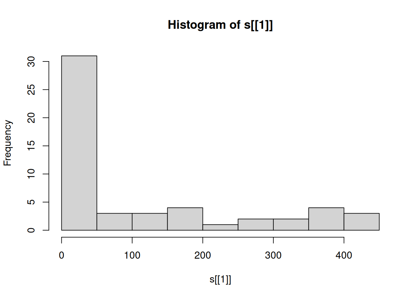
Figure 5.17: Distribution of elevation values

For example, the above histogram tells us that the overall range of elevation values in the raster s is roughly 0-450 (\(m\)), but most pixels are in the 0-50 \(m\) elevation range.

Note that we can pass the matrix (or array) of raster values to many other functions that accept a numeric vector, such as mean or range.

Calculate the mean, minimum and maximum of the cell values in the raster s (excluding NA).

The matrix or array rows and columns are swapped, compared to the visual arrangement of the raster, because in a stars object the first dimension (matrix rows) refers to x (raster columns) and the second dimension (matrix columns) refers to y (raster rows)! For example, the following expression returns the 7^th column of the matrix that holds the raster values, which actually refers to the 7^th row in terms of the spatial arrangement of the raster (Figure 5.15):

s[[1]][, 7]
## [1]  NA  31 233 340 163  13  64

We can modify (a subset of) raster values using assignment. For example, the following code creates a copy of the raster s, named u, then replaces the values in the 7^th row (of the raster) with the value -1:

u = s
u[[1]][, 7] = -1

The resulting raster u is shown in Figure 5.18:

plot(u, text_values = TRUE, axes = TRUE, col = terrain.colors(8))

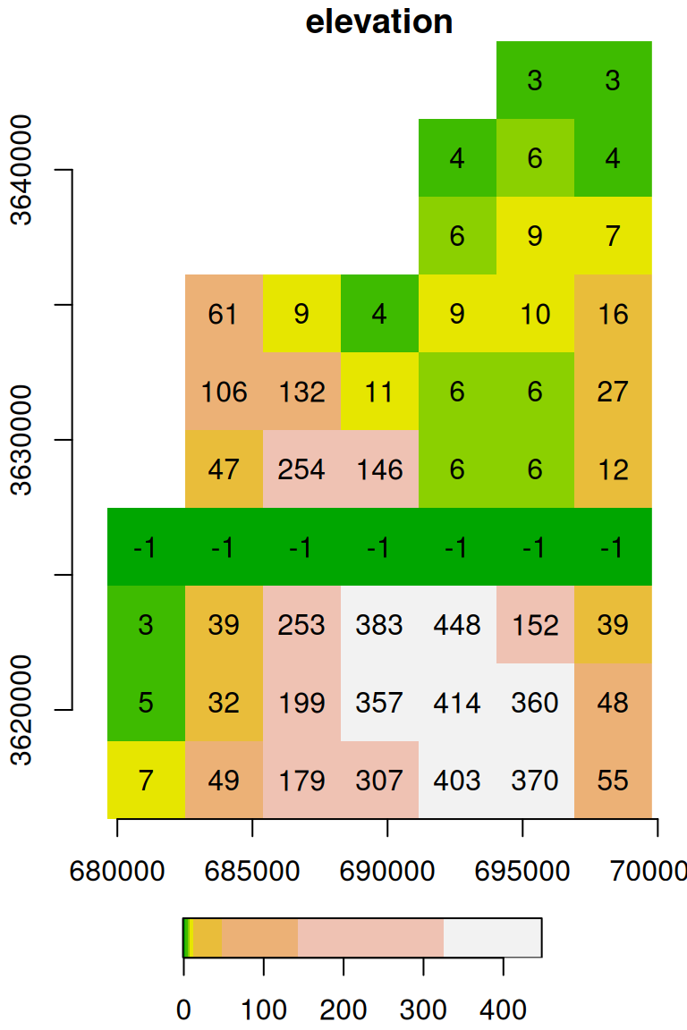
Figure 5.18: Raster with the value -1 assigned into the 7th row

We can even replace the entire matrix or array of values with a custom one. This can be done using assignment to an “empty” subset, which implies selecting all cells, as in r[[1]][]. For example, the following code section creates another copy named u, then replaces all values with a consecutive vector:

u = s
u[[1]][] = 1:length(u[[1]])
u[[1]]
##      [,1] [,2] [,3] [,4] [,5] [,6] [,7] [,8] [,9] [,10]
## [1,]    1    8   15   22   29   36   43   50   57    64
## [2,]    2    9   16   23   30   37   44   51   58    65
## [3,]    3   10   17   24   31   38   45   52   59    66
## [4,]    4   11   18   25   32   39   46   53   60    67
## [5,]    5   12   19   26   33   40   47   54   61    68
## [6,]    6   13   20   27   34   41   48   55   62    69
## [7,]    7   14   21   28   35   42   49   56   63    70

The resulting raster u is shown in Figure 5.19:

plot(u, text_values = TRUE, axes = TRUE, breaks = 'equal', col = terrain.colors(30))

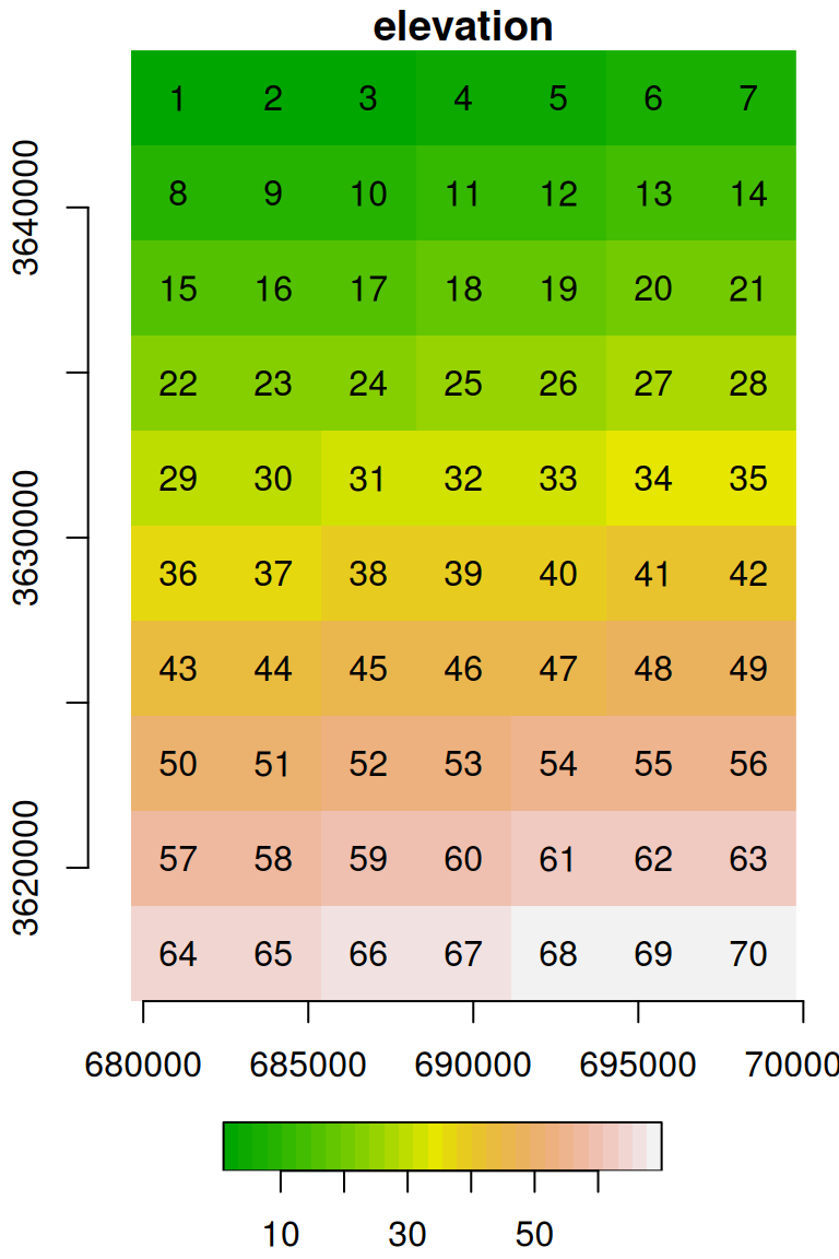
Figure 5.19: Raster with consecutive values

Sometimes it is useful to assign the same value to all cells, to create a uniform raster. This can be done using assignment of a single value, which is replicated, to the subset of all raster cells:

u = s
u[[1]][] = -3
u[[1]]
##      [,1] [,2] [,3] [,4] [,5] [,6] [,7] [,8] [,9] [,10]
## [1,]   -3   -3   -3   -3   -3   -3   -3   -3   -3    -3
## [2,]   -3   -3   -3   -3   -3   -3   -3   -3   -3    -3
## [3,]   -3   -3   -3   -3   -3   -3   -3   -3   -3    -3
## [4,]   -3   -3   -3   -3   -3   -3   -3   -3   -3    -3
## [5,]   -3   -3   -3   -3   -3   -3   -3   -3   -3    -3
## [6,]   -3   -3   -3   -3   -3   -3   -3   -3   -3    -3
## [7,]   -3   -3   -3   -3   -3   -3   -3   -3   -3    -3

The resulting raster u is shown in Figure 5.20:

plot(u, text_values = TRUE, axes = TRUE, breaks = 'equal', col = terrain.colors(1))

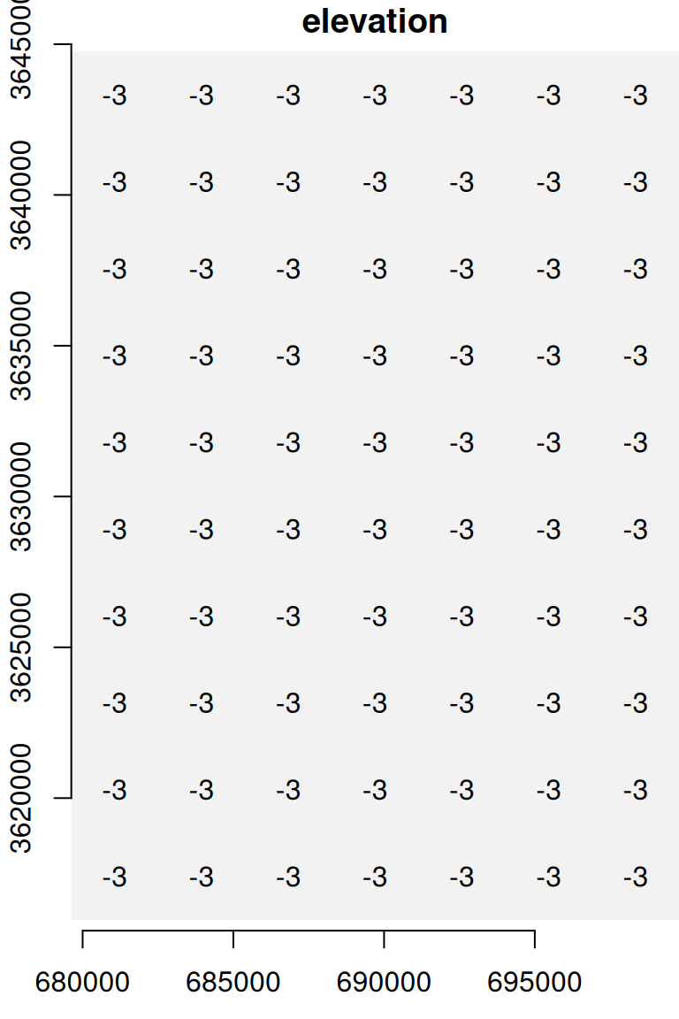
Figure 5.20: A uniform raster

5.3.9 Writing raster to file

We will not need to export rasters (or vector layers) in this book, since we will be working exclusively in the R environment. In practice, however, one often needs to export spatial objects from R to a file, to share them with other colleagues, further edit or process them in GIS software such as ArcGIS or QGIS, and so on.

Writing a stars raster object to a file on disk is done using write_stars. To run write_stars, we need to specify:

• obj—The stars object to write
• dsn—The file name (or file path) of the raster file being created

The function can automatically detect the required file format based on the file extension. For example, the following expression exports the stars object named s to a GeoTIFF file named dem_copy.tif in the current working directory:

write_stars(s, 'dem_copy.tif')

References

Wickham, Hadley et al. 2011. “The Split-Apply-Combine Strategy for Data Analysis.” Journal of Statistical Software 40 (1): 1–29.

---

17. Due to the conventions of image, a matrix image is actually reversed in 90 degrees compared to the textual representation of a matrix. To get the same orientation as in the textual representation, use image(t(apply(volcano,2,rev)))↩︎

18. There are similar functions named rowSums and colSums for calculating row and column sums, respectively.↩︎

19. Note that there are no data structure for zero-dimensional data structures (i.e., scalars) in R.↩︎

20. https://en.wikipedia.org/wiki/Null_Island↩︎

21. Unless a new version of a package was released and we want to update it, in which case we need to re-install the package.↩︎

22. GeoTIFF files can come with both *.tif and *.tiff file extension, so if one of them does not work you should try the other.↩︎