Chapter 13 Point pattern analysis (in preparation)

Last updated: 2023-05-03 11:15:27

Aims

Our aims in this chapter are:

We will use the following R packages:

spatstat
sf
stars

13.1 Introduction

A point pattern dataset gives the locations of objects/events occurring in a study region. For examples, mapped occurence of the following objects or events can comprise a point pattern:

Trees
Animal nests
Earthquake epicentres
Crime cases
Galaxies

The points may have extra information, called marks, attached to them. Our dataset may also include covariates, any data that we treat as explanatory, rather than as part of the “response”.

Scientific questions:

Intensity - Average density of points
Interaction - Dependence between points
Covariate effects - Whether the intensity depends on covariates
Segregation of points with different marks
Dependence between points of different types

We are going to demonstrate point pattern analysis using the spatstat package.

13.2 Data

The spatstat package comes with several sample datasets, including:

cells - Biological Cells Point Pattern
japanesepines - Japanese Pines Point Pattern
redwood - California Redwoods Point Pattern

Printing a point pattern object shows some basic properties, including the number of points and the type of “window”. For example:

library(spatstat)
cells
## Planar point pattern: 42 points
## window: rectangle = [0, 1] x [0, 1] units
japanesepines
## Planar point pattern: 65 points
## window: rectangle = [0, 1] x [0, 1] units (one unit = 5.7 metres)
redwood
## Planar point pattern: 62 points
## window: rectangle = [0, 1] x [-1, 0] units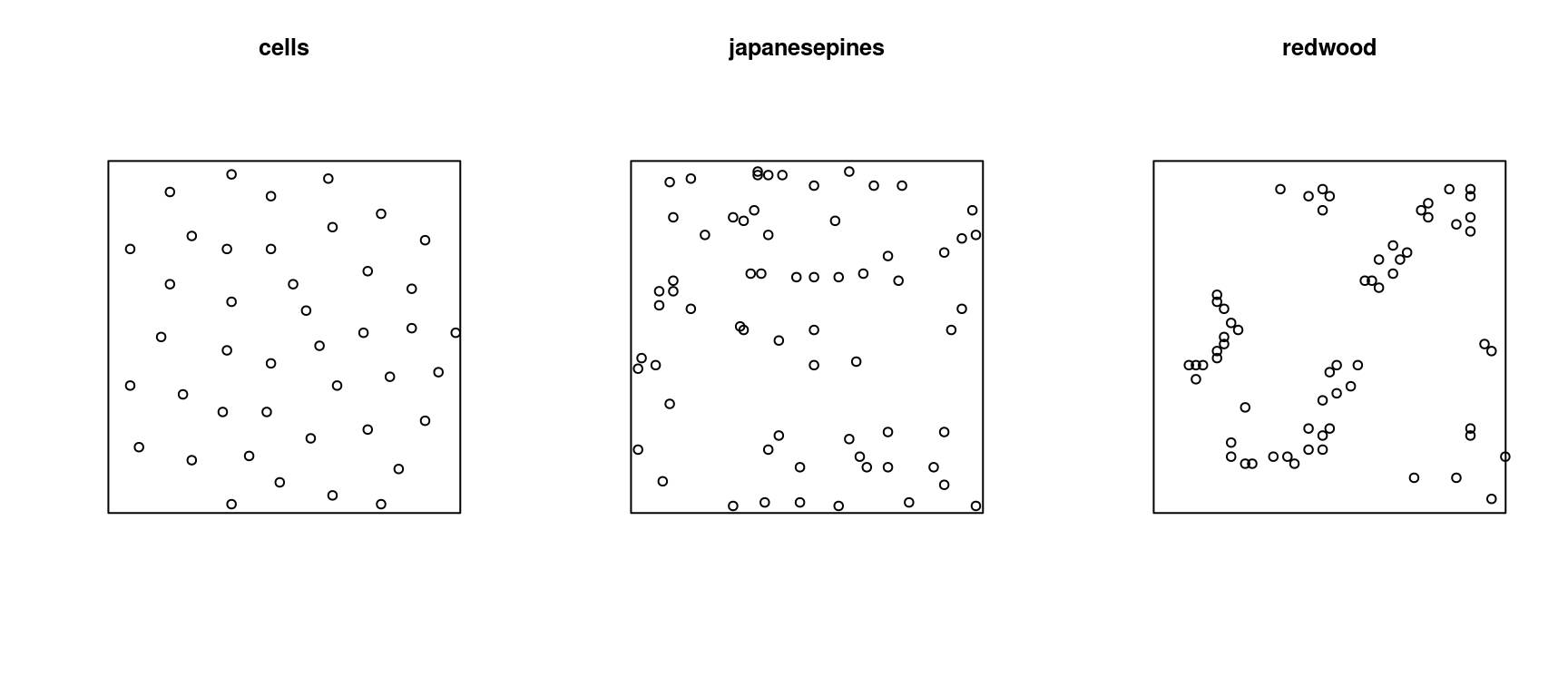

Figure 13.1: Distance map for the Biological Cells Point Pattern dataset

We will use two vector layers:

reserve—Boundaries of the “Negev Mountain” nature reserve
plants—Location of rare plant observations

library(sf)
reserve = st_read("reserve.shp")
plants = st_read("plants.shp")

Let us transform to a projected CRS (UTM):

reserve = st_transform(reserve, 32636)
plants = st_transform(plants, 32636)

Plot.

plot(st_geometry(reserve))
plot(st_geometry(plants), add = TRUE, col = "red")

13.3 Preparing point pattern data

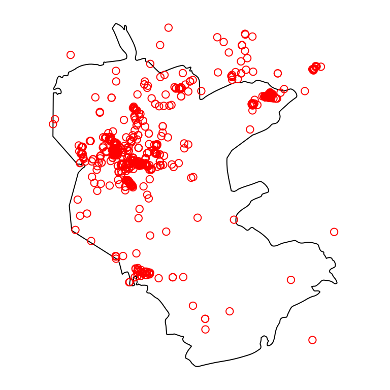
Figure 13.2: Nature reserve and rare plants observations

We subset only those plants that were observed within the reserve:

plants = plants[reserve, ]

plot(st_geometry(reserve))
plot(st_geometry(plants), add = TRUE, col = "red")

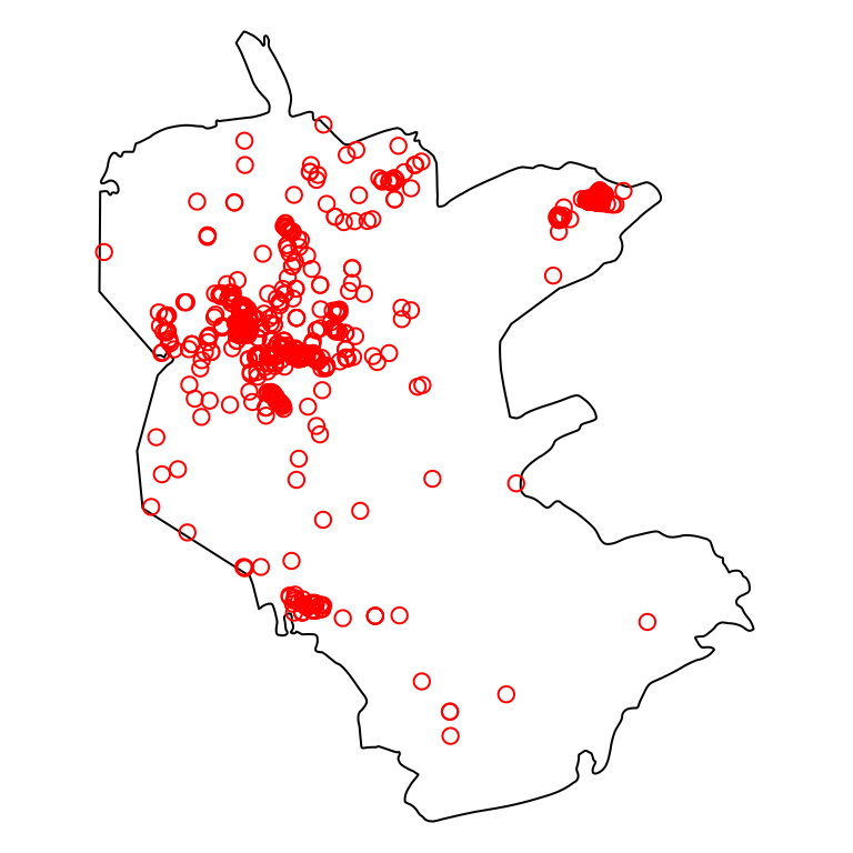
Figure 13.3: Nature reserve and rare plants observations (subset)

Then we convert from sf to a ppp point pattern object, using function as.ppp:

pnt = st_geometry(plants)
pnt = as.ppp(pnt)

pnt
## Planar point pattern: 816 points
## window: rectangle = [646200, 679754.5] x [3351394, 3389148] units

Plot.

plot(pnt)

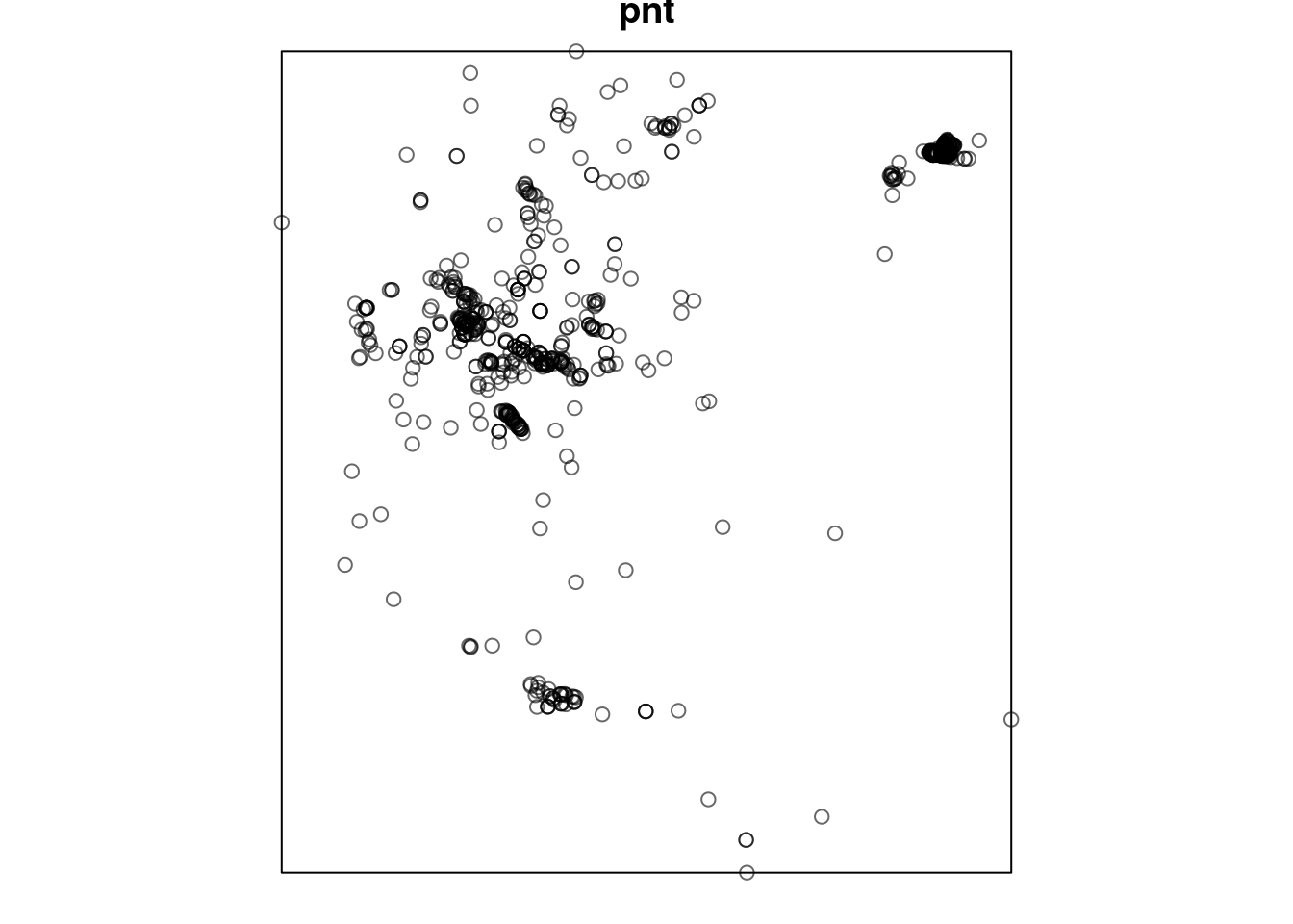
Figure 13.4: Plant observations point pattern as a ppp object

The reserve polygon represents the area where the phenomenon is completely mapped. It can be converted to an owin (“observation window”) object:

pol = st_geometry(reserve)
pol = as.owin(pol)

pol
## window: polygonal boundary
## enclosing rectangle: [645913.1, 686312.6] x [3346117, 3394893] units

Plot.

plot(pol)

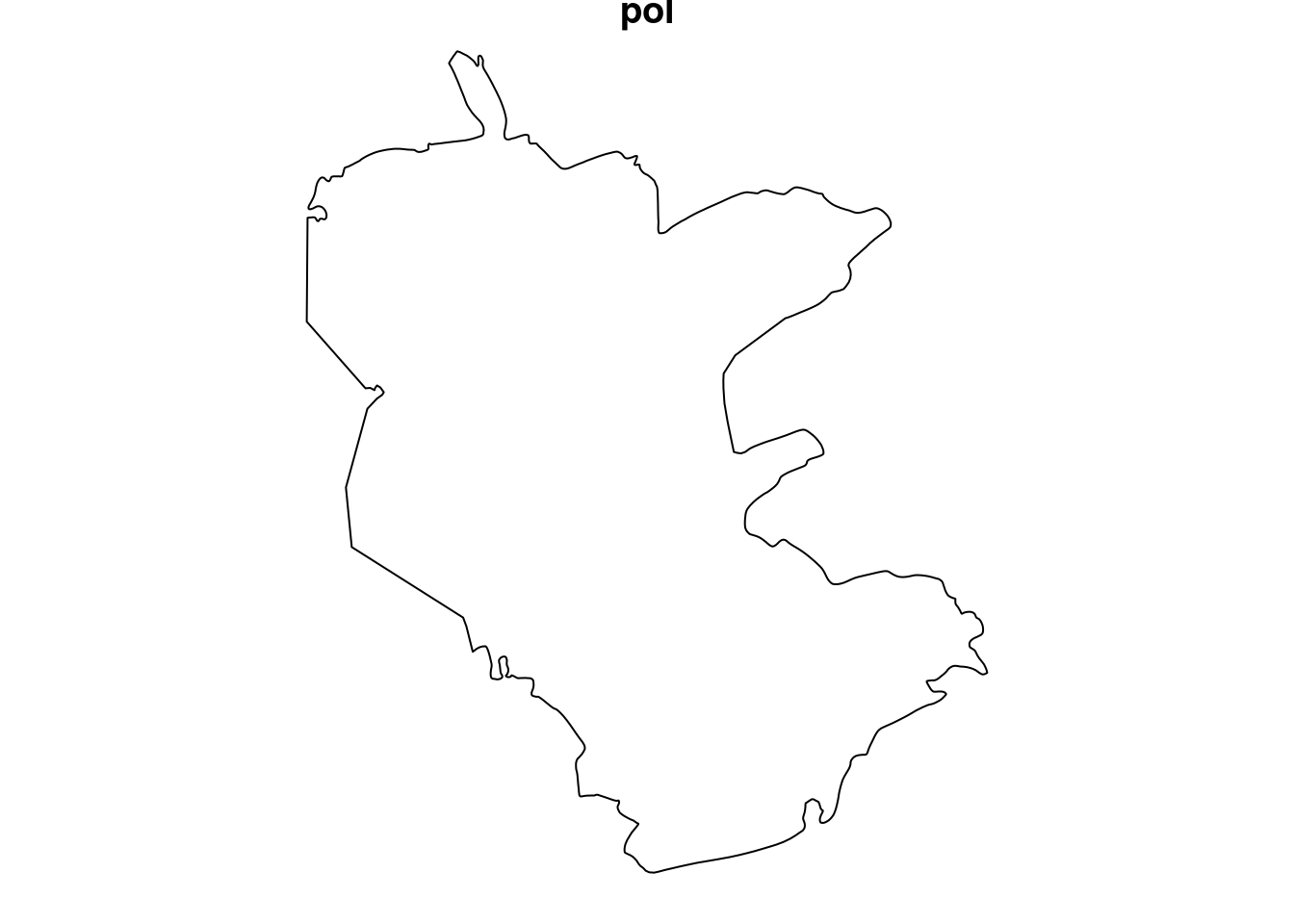
Figure 13.5: Observation window

The observation window and the point pattern can be combined, so that the custom window replaces the default ractangular extent:

pnt = pnt[pol]
pnt
## Planar point pattern: 816 points
## window: polygonal boundary
## enclosing rectangle: [645913.1, 686312.6] x [3346117, 3394893] units

Plot.

plot(pnt)

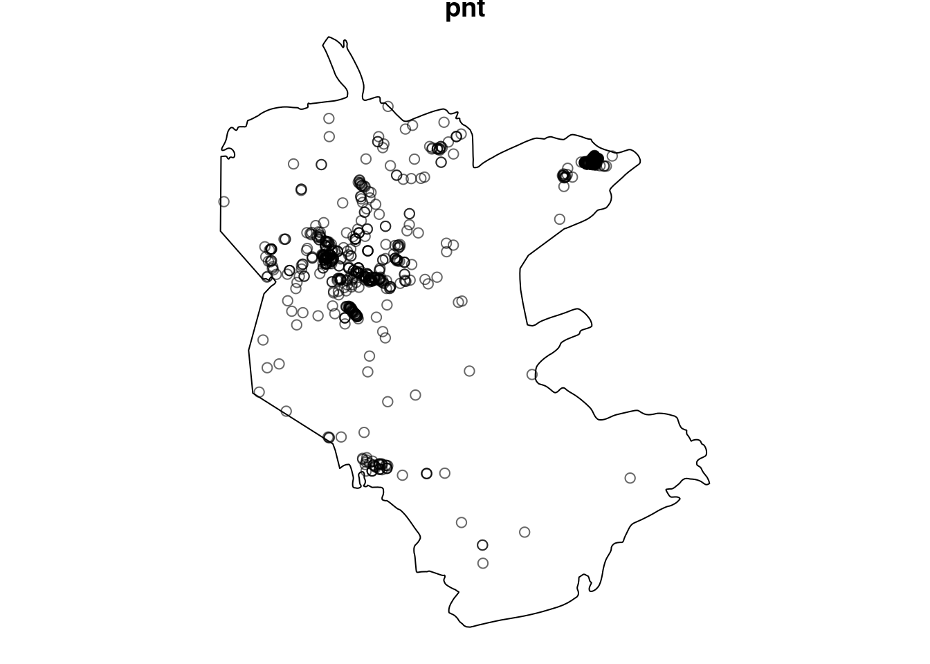
Figure 13.6: Point pattern with custom observation window

13.4 Density estimation

q = quadratcount(pnt, nx = 7, ny = 7)

plot(q)

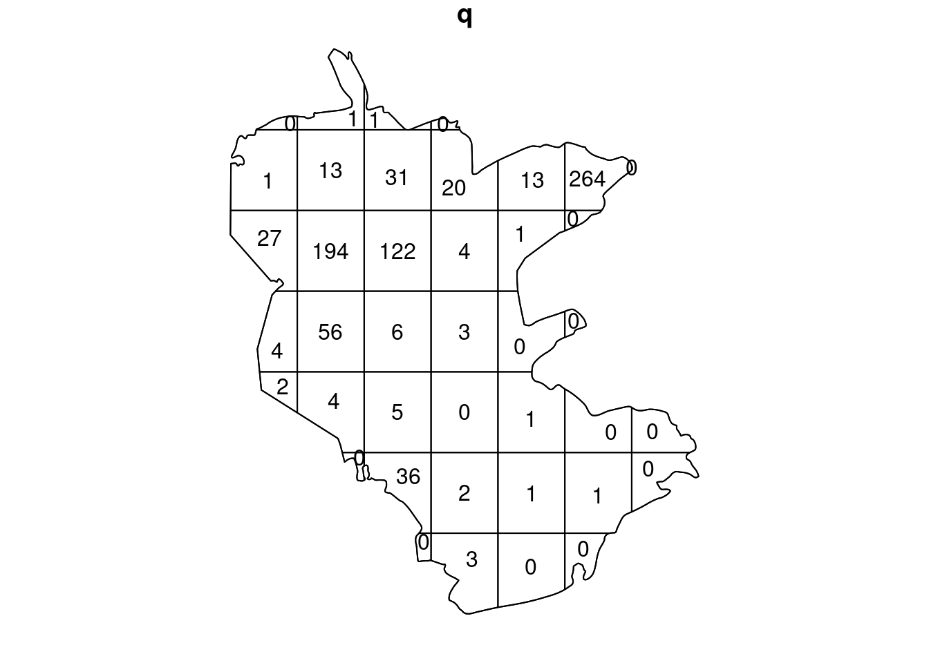
quadrat.test(pnt, nx = 7, ny = 7)
## Warning: Some expected counts are small; chi^2 approximation may be inaccurate
## 
##  Chi-squared test of CSR using quadrat counts
## 
## data:  pnt
## X2 = 4935.6, df = 39, p-value < 2.2e-16
## alternative hypothesis: two.sided
## 
## Quadrats: 40 tiles (irregular windows)

Kernel density estimation of a point pattern can be done using function density:

den = density(pnt)
den
## real-valued pixel image
## 128 x 128 pixel array (ny, nx)
## enclosing rectangle: [645910, 686310] x [3346100, 3394900] units

Plot -

plot(den, main = "")
plot(pnt, pch = 1, cex = 0.5, add = TRUE)
contour(den, add = TRUE)

$Plant observation density, \texttt{im} object$

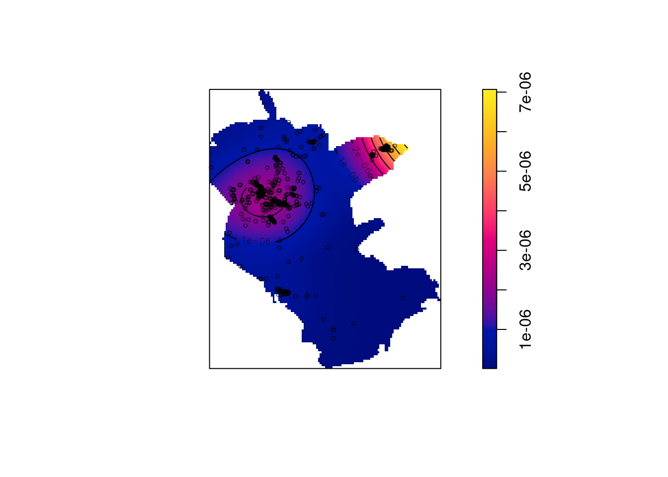
Figure 13.7: Plant observation density, object

The resulting object of class im (image) can be converted to a raster with raster:

library(raster)
## 
## Attaching package: 'raster'
## The following object is masked from 'package:dplyr':
## 
##     select
## The following object is masked from 'package:nlme':
## 
##     getData
library(stars)
r = raster(den)
r = st_as_stars(r)
r
## stars object with 2 dimensions and 1 attribute
## attribute(s):
##                Min.      1st Qu.       Median         Mean      3rd Qu.
## layer  1.169344e-08 8.771615e-08 5.313579e-07 7.899422e-07 1.126727e-06
##               Max. NA's
## layer  7.06921e-06 7958
## dimension(s):
##   from  to  offset    delta x/y
## x    1 128  645913  315.621 [x]
## y    1 128 3394893 -381.064 [y]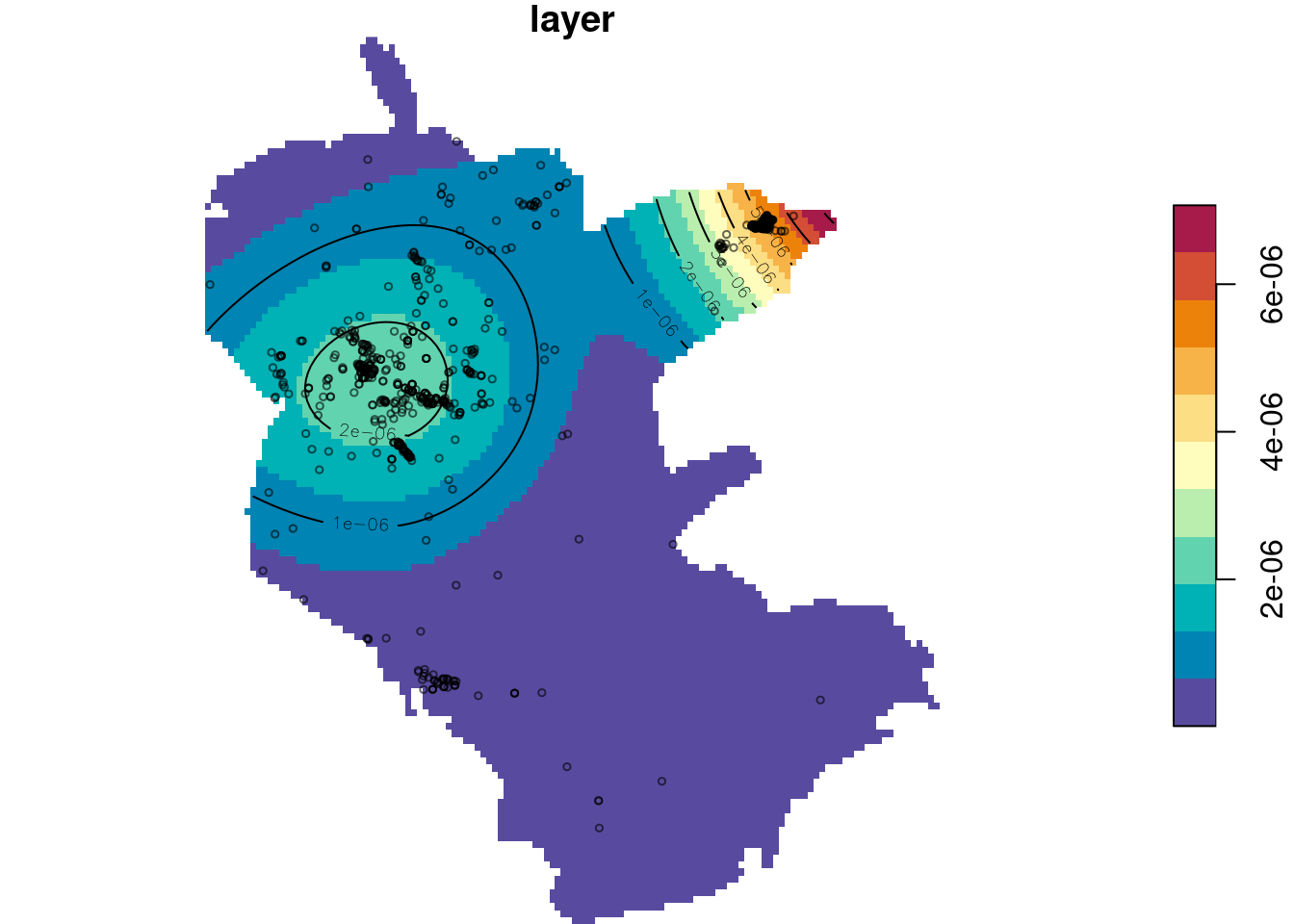

Figure 13.8: Plant observation density, as stars object

We can change the standard deviation of the kernel using sigma:

den = density(pnt, sigma = 2000)

plot(den)
plot(pnt, pch = 1, cex = 0.5, add = TRUE)
contour(den, add = TRUE)

$Plant observation density, manually setting \texttt{sigma}$

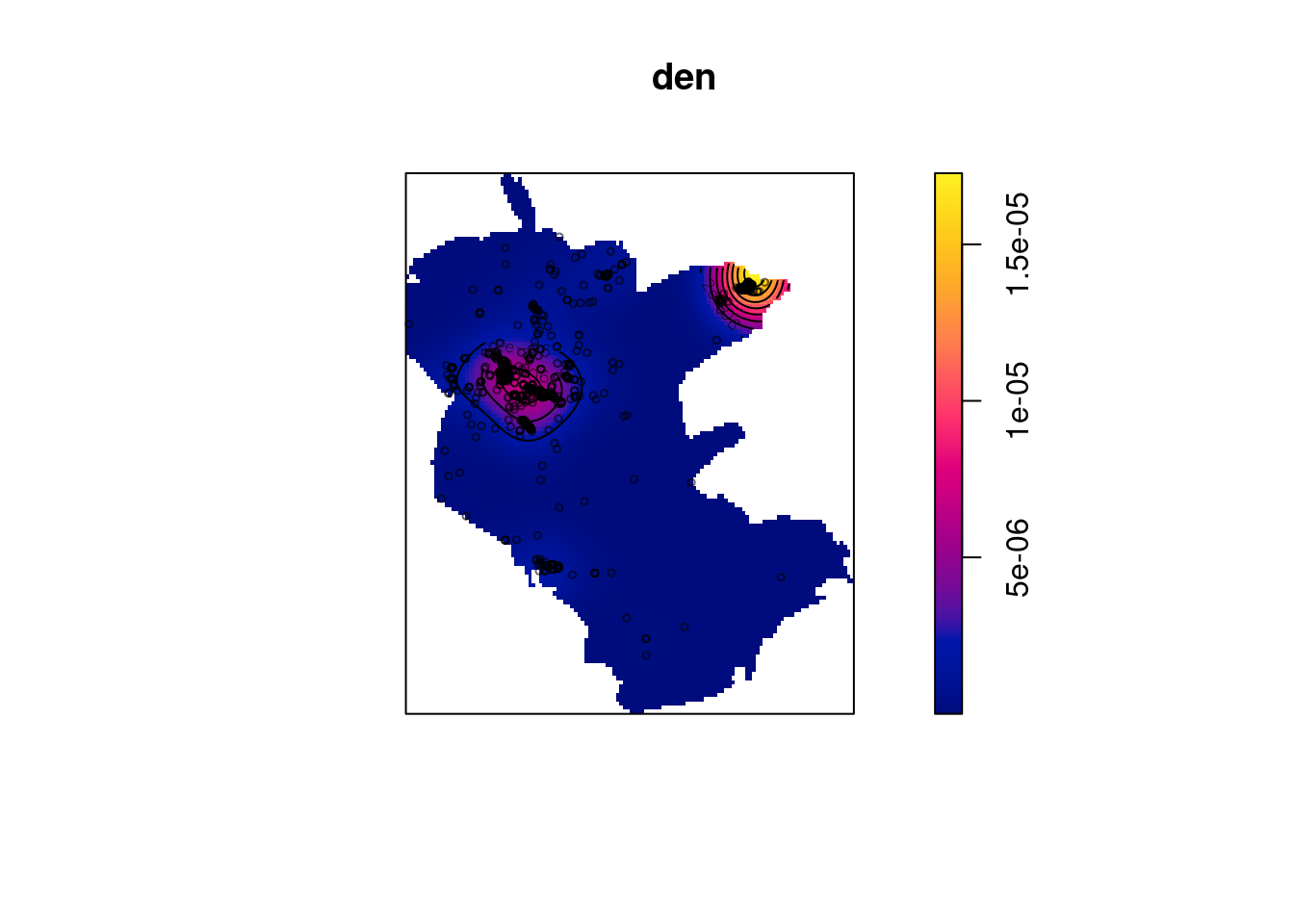
Figure 13.9: Plant observation density, manually setting

13.5 Pattern type

Ripley’s K-function measures the expected number of random points within a distance $r$ of a typical random point of a point pattern $X$.

Kcells = envelope(cells, fun = Kest)
Kpines = envelope(japanesepines, fun = Kest)
Kredwood = envelope(redwood, fun = Kest)

Kcells = envelope(cells, fun = Kest)
## Generating 99 simulations of CSR  ...
## 1, 2, 3, 4, 5, 6, 7, 8, 9, 10, 11, 12, 13, 14, 15, 16, 17, 18, 19, 20, 21, 22, 23, 24, 25, 26, 27, 28, 29, 30, 31, 32, 33, 34, 35, 36, 37, 38, 39, 40,
## 41, 42, 43, 44, 45, 46, 47, 48, 49, 50, 51, 52, 53, 54, 55, 56, 57, 58, 59, 60, 61, 62, 63, 64, 65, 66, 67, 68, 69, 70, 71, 72, 73, 74, 75, 76, 77, 78, 79, 80,
## 81, 82, 83, 84, 85, 86, 87, 88, 89, 90, 91, 92, 93, 94, 95, 96, 97, 98,  99.
## 
## Done.
Kpines = envelope(japanesepines, fun = Kest)
## Generating 99 simulations of CSR  ...
## 1, 2, 3, 4, 5, 6, 7, 8, 9, 10, 11, 12, 13, 14, 15, 16, 17, 18, 19, 20, 21, 22, 23, 24, 25, 26, 27, 28, 29, 30, 31, 32, 33, 34, 35, 36, 37, 38, 39, 40,
## 41, 42, 43, 44, 45, 46, 47, 48, 49, 50, 51, 52, 53, 54, 55, 56, 57, 58, 59, 60, 61, 62, 63, 64, 65, 66, 67, 68, 69, 70, 71, 72, 73, 74, 75, 76, 77, 78, 79, 80,
## 81, 82, 83, 84, 85, 86, 87, 88, 89, 90, 91, 92, 93, 94, 95, 96, 97, 98,  99.
## 
## Done.
Kredwood = envelope(redwood, fun = Kest)
## Generating 99 simulations of CSR  ...
## 1, 2, 3, 4, 5, 6, 7, 8, 9, 10, 11, 12, 13, 14, 15, 16, 17, 18, 19, 20, 21, 22, 23, 24, 25, 26, 27, 28, 29, 30, 31, 32, 33, 34, 35, 36, 37, 38, 39, 40,
## 41, 42, 43, 44, 45, 46, 47, 48, 49, 50, 51, 52, 53, 54, 55, 56, 57, 58, 59, 60, 61, 62, 63, 64, 65, 66, 67, 68, 69, 70, 71, 72, 73, 74, 75, 76, 77, 78, 79, 80,
## 81, 82, 83, 84, 85, 86, 87, 88, 89, 90, 91, 92, 93, 94, 95, 96, 97, 98,  99.
## 
## Done.

plot(Kcells)
plot(Kpines)
plot(Kredwood)

Ripley’s K envelope plots are interpreted as follows:

Observed $K(r)$ values below the envelope indicate lower than exprected density at radius $r$, i.e., significant sparseness.
Observed $K(r)$ values within the envelope indicate no significant deviation from sparseness.
Observed $K(r)$ values above the envelope indicate higher than exprected density at radius $r$, i.e., significant clustering.

Accordingly, we conclude that:

The cells point pattern is significantly sparse at short distances, i.e., follows a regular pattern
The pines point pattern is random
The redwood point pattern is significanly clustered at short to medium distances

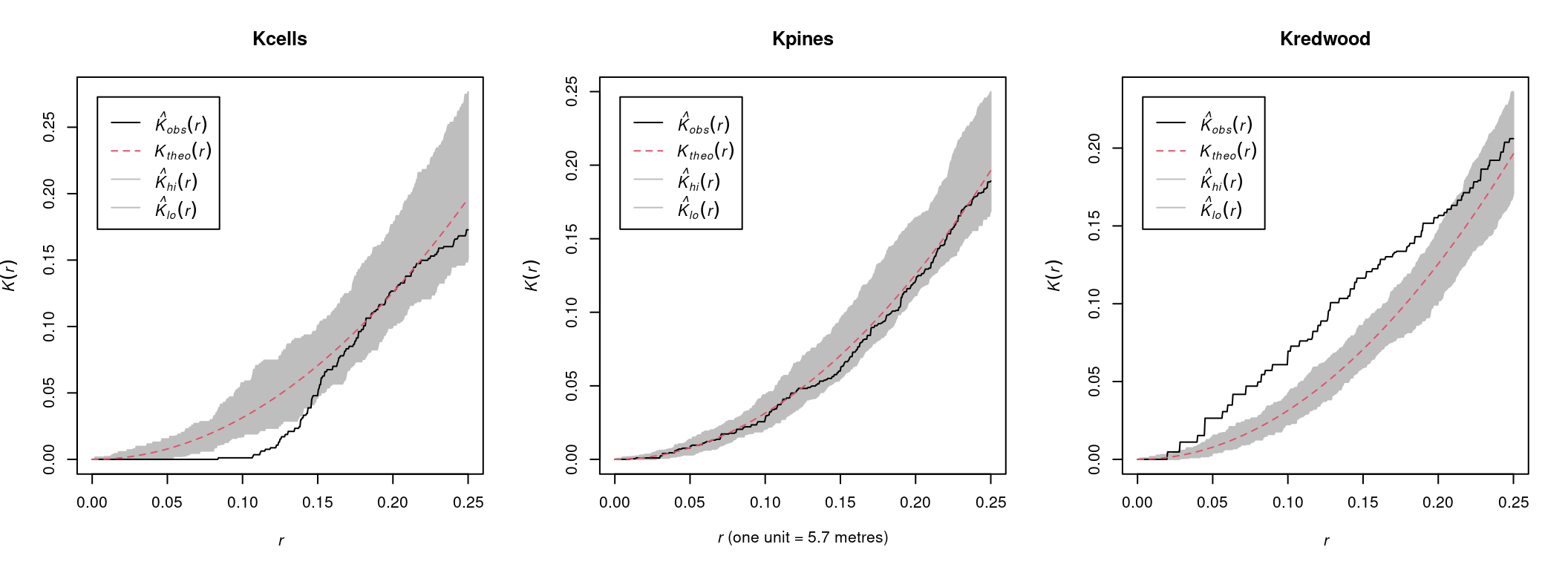
Figure 13.10: Ripley’s K functions for the cells, pines and redwood datasets.

k = Kest(pnt)

plot(k)

Figure 13.11: Ripley’s K function for the plants dataset

Generating envelope…

e = envelope(pnt, fun = Kest)
## Generating 99 simulations of CSR  ...
## 1, 2,  [etd 11:26] 3,  [etd 10:36] 4,
##  [etd 10:45] 5,  [etd 10:23] 6,  [etd 10:17] 7,  [etd 10:00] 8,
##  [etd 10:06] 9,  [etd 10:00] 10,  [etd 10:05] 11,  [etd 9:55] 12,
##  [etd 9:51] 13,  [etd 9:43] 14,  [etd 9:40] 15,  [etd 9:35] 16,
##  [etd 9:28] 17,  [etd 9:29] 18,  [etd 9:28] 19,  [etd 9:21] 20,
##  [etd 9:16] 21,  [etd 9:13] 22,  [etd 9:08] 23,  [etd 9:04] 24,
##  [etd 9:00] 25,  [etd 8:53] 26,  [etd 8:46] 27,  [etd 8:40] 28,
##  [etd 8:33] 29,  [etd 8:28] 30,  [etd 8:20] 31,  [etd 8:12] 32,
##  [etd 8:06] 33,  [etd 7:57] 34,  [etd 7:50] 35,  [etd 7:42] 36,
##  [etd 7:34] 37,  [etd 7:28] 38,  [etd 7:20] 39,  [etd 7:13] 40,
##  [etd 7:05] 41,  [etd 6:59] 42,  [etd 6:53] 43,  [etd 6:48] 44,
##  [etd 6:42] 45,  [etd 6:36] 46,  [etd 6:30] 47,  [etd 6:23] 48,
##  [etd 6:15] 49,  [etd 6:08] 50,  [etd 6:01] 51,  [etd 5:54] 52,
##  [etd 5:47] 53,  [etd 5:40] 54,  [etd 5:32] 55,  [etd 5:24] 56,
##  [etd 5:17] 57,  [etd 5:09] 58,  [etd 5:02] 59,  [etd 4:55] 60,
##  [etd 4:47] 61,  [etd 4:40] 62,  [etd 4:33] 63,  [etd 4:25] 64,
##  [etd 4:18] 65,  [etd 4:11] 66,  [etd 4:03] 67,  [etd 3:56] 68,
##  [etd 3:49] 69,  [etd 3:41] 70,  [etd 3:34] 71,  [etd 3:26] 72,
##  [etd 3:19] 73,  [etd 3:12] 74,  [etd 3:05] 75,  [etd 2:57] 76,
##  [etd 2:50] 77,  [etd 2:42] 78,  [etd 2:35] 79,  [etd 2:28] 80,
##  [etd 2:21] 81,  [etd 2:13] 82,  [etd 2:06] 83,  [etd 1:58] 84,
##  [etd 1:51] 85,  [etd 1:44] 86,  [etd 1:36] 87,  [etd 1:29] 88,
##  [etd 1:22] 89,  [etd 1:14] 90,  [etd 1:07] 91,  [etd 1:00] 92,
##  [etd 52 sec] 93,  [etd 45 sec] 94,  [etd 37 sec] 95,  [etd 30 sec] 96,
##  [etd 22 sec] 97,  [etd 15 sec] 98,  [etd 7 sec]  99.
## 
## Done.

Plot.

plot(e)

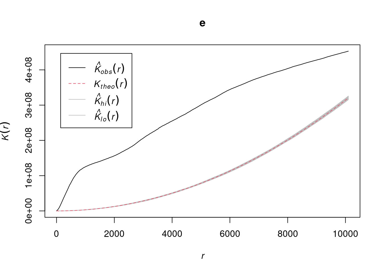
Figure 13.12: Ripley’s K function for the plants dataset, with an envelope

13.6 Models

13.6.1 Model fitting

Model fitting…

fit0 = ppm(pnt, ~1)

Model summary…

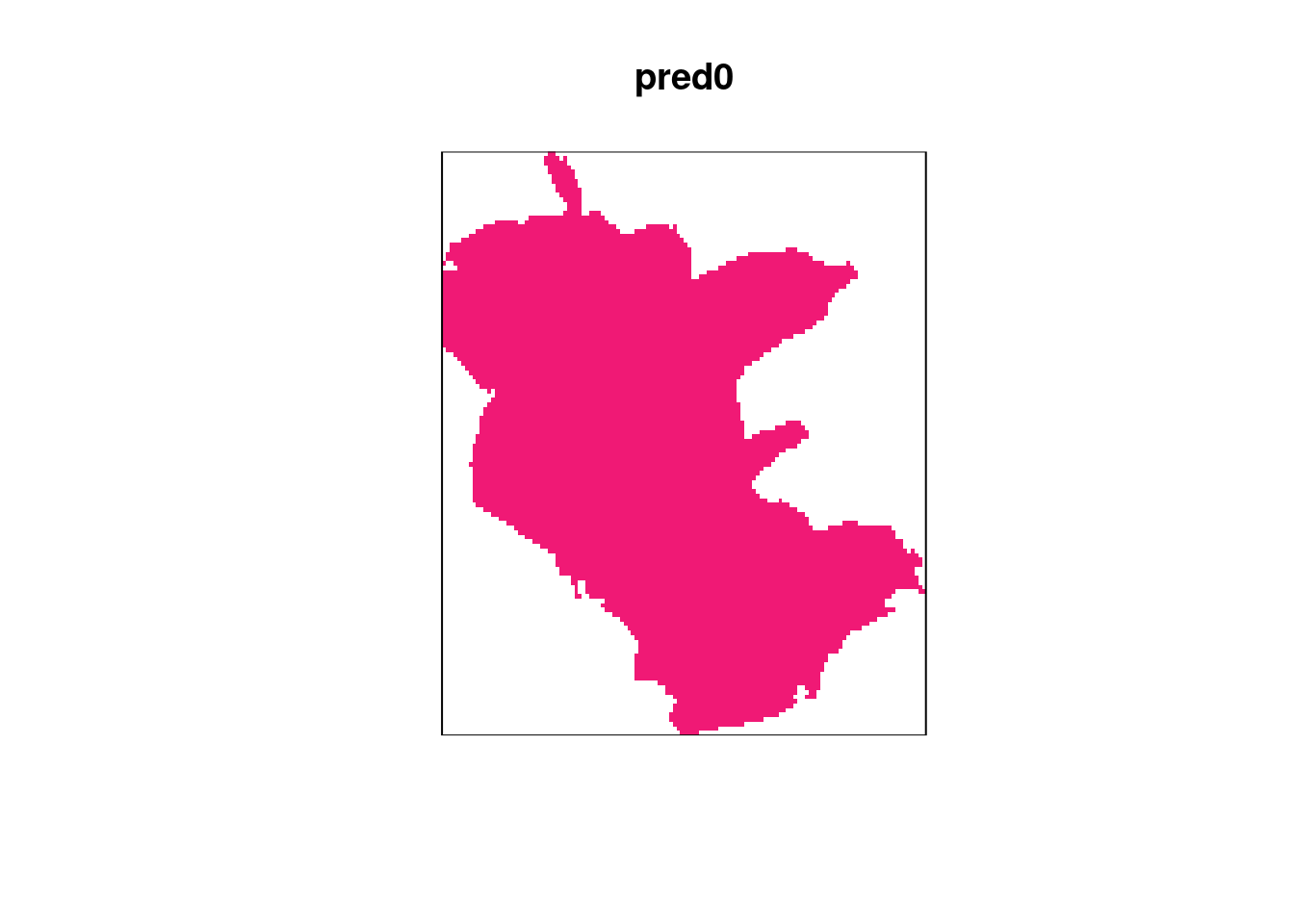
summary(fit0)
## Point process model
## Fitted to data: pnt
## Fitting method: maximum likelihood
## Model was fitted analytically
## Call:
## ppm.ppp(Q = pnt, trend = ~1)
## Edge correction: "border"
##  [border correction distance r = 0 ]
## --------------------------------------------------------------------------------
## Quadrature scheme (Berman-Turner) = data + dummy + weights
## 
## Data pattern:
## Planar point pattern:  816 points
## Average intensity 8.05e-07 points per square unit
## Window: polygonal boundary
## single connected closed polygon with 1269 vertices
## enclosing rectangle: [645913.1, 686312.6] x [3346117, 3394893] units
##                      (40400 x 48780 units)
## Window area = 1014220000 square units
## Fraction of frame area: 0.515
## 
## Dummy quadrature points:
##      64 x 64 grid of dummy points, plus 4 corner points
##      dummy spacing: 631.2419 x 762.1274 units
## 
## Original dummy parameters: =
## Planar point pattern:  2191 points
## Average intensity 2.16e-06 points per square unit
## Window: polygonal boundary
## single connected closed polygon with 1269 vertices
## enclosing rectangle: [645913.1, 686312.6] x [3346117, 3394893] units
##                      (40400 x 48780 units)
## Window area = 1014220000 square units
## Fraction of frame area: 0.515
## Quadrature weights:
##      (counting weights based on 64 x 64 array of rectangular tiles)
## All weights:
##  range: [2830, 481000]   total: 1.01e+09
## Weights on data points:
##  range: [2830, 241000]   total: 56900000
## Weights on dummy points:
##  range: [2830, 481000]   total: 9.55e+08
## --------------------------------------------------------------------------------
## FITTED :
## 
## Stationary Poisson process
## 
## ---- Intensity: ----
## 
## 
## Uniform intensity:
## [1] 8.045619e-07
## 
##              Estimate     S.E.   CI95.lo   CI95.hi Ztest      Zval
## log(lambda) -14.03297 0.035007 -14.10158 -13.96436   *** -400.8617
## 
## ----------- gory details -----
## 
## Fitted regular parameters (theta):
## log(lambda) 
##   -14.03297 
## 
## Fitted exp(theta):
##  log(lambda) 
## 8.045619e-07

13.6.2 Preparing covariate data

elev = read_stars("_book/data/reserve_elev.tif")

plot(st_geometry(reserve), border = NA)
plot(elev, add = TRUE)
plot(st_geometry(reserve), add = TRUE)
plot(st_geometry(plants), add = TRUE, col = "red")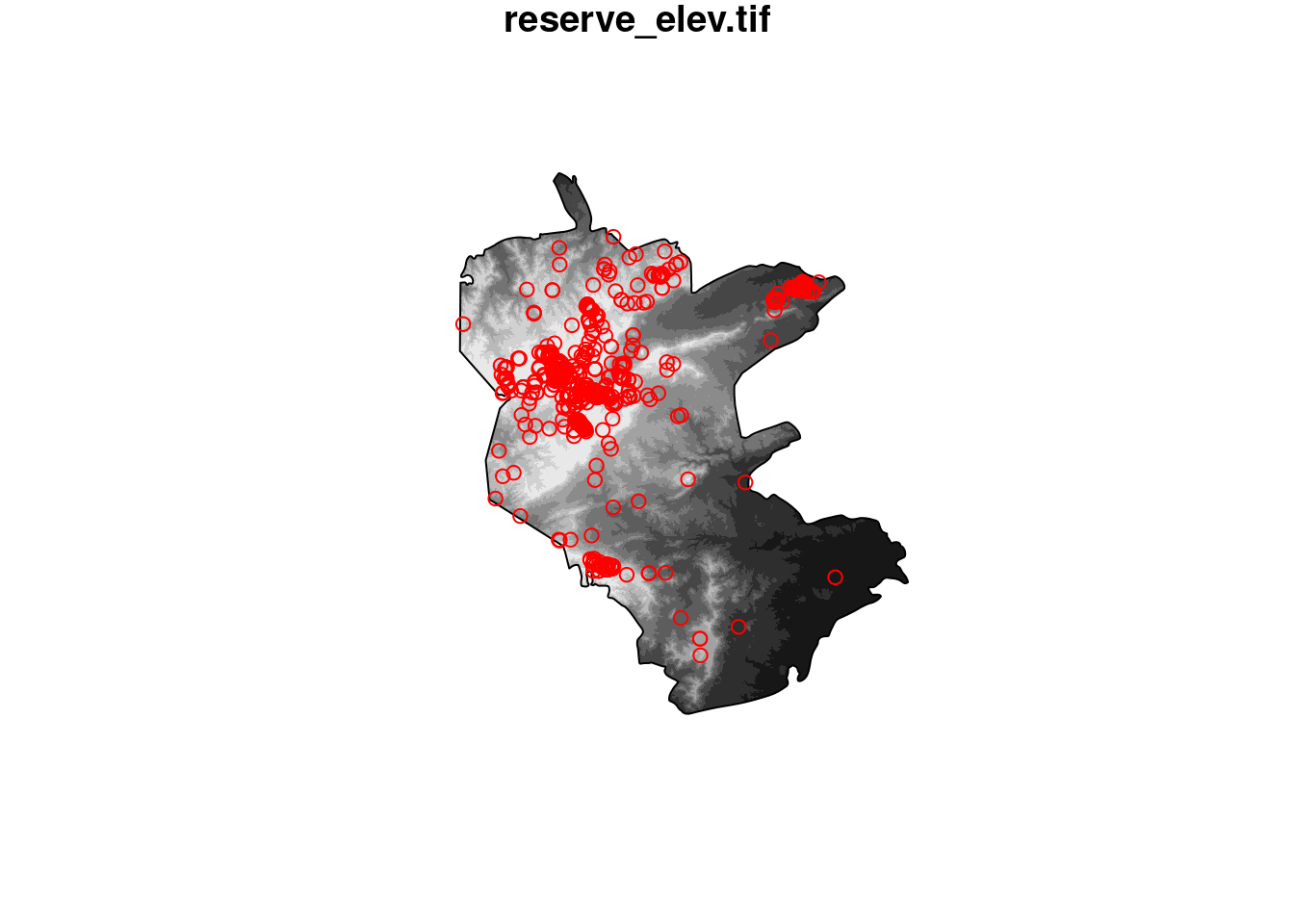

elev = as.im(elev)

Plot.

plot(elev)

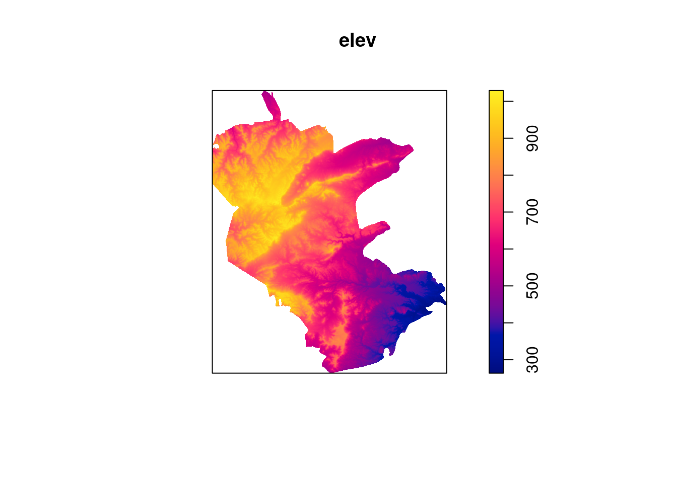
13.6.3 Model with covariates

Model fitting…

fit1 = ppm(pnt, ~elev)

Model summary…

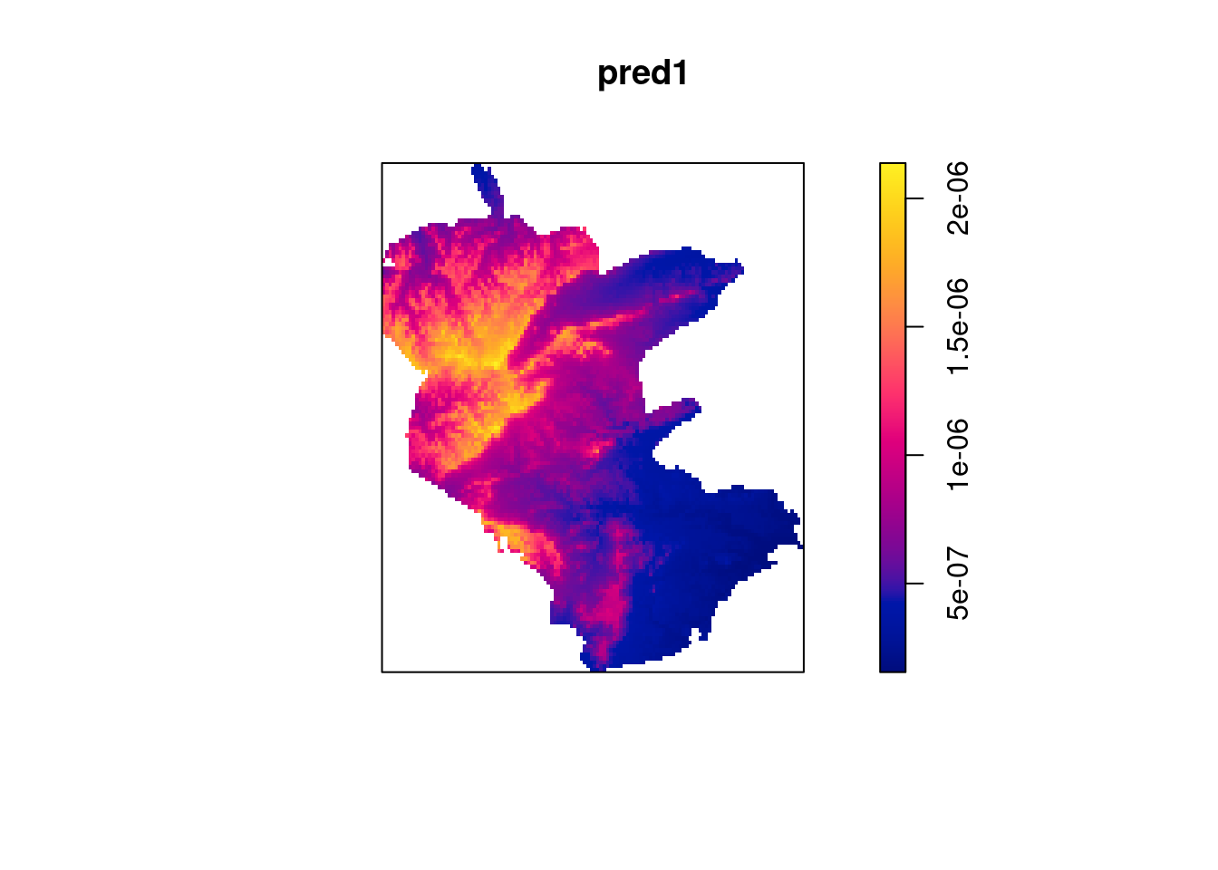
summary(fit1)
## Point process model
## Fitted to data: pnt
## Fitting method: maximum likelihood (Berman-Turner approximation)
## Model was fitted using glm()
## Algorithm converged
## Call:
## ppm.ppp(Q = pnt, trend = ~elev)
## Edge correction: "border"
##  [border correction distance r = 0 ]
## --------------------------------------------------------------------------------
## Quadrature scheme (Berman-Turner) = data + dummy + weights
## 
## Data pattern:
## Planar point pattern:  816 points
## Average intensity 8.05e-07 points per square unit
## Window: polygonal boundary
## single connected closed polygon with 1269 vertices
## enclosing rectangle: [645913.1, 686312.6] x [3346117, 3394893] units
##                      (40400 x 48780 units)
## Window area = 1014220000 square units
## Fraction of frame area: 0.515
## 
## Dummy quadrature points:
##      64 x 64 grid of dummy points, plus 4 corner points
##      dummy spacing: 631.2419 x 762.1274 units
## 
## Original dummy parameters: =
## Planar point pattern:  2191 points
## Average intensity 2.16e-06 points per square unit
## Window: polygonal boundary
## single connected closed polygon with 1269 vertices
## enclosing rectangle: [645913.1, 686312.6] x [3346117, 3394893] units
##                      (40400 x 48780 units)
## Window area = 1014220000 square units
## Fraction of frame area: 0.515
## Quadrature weights:
##      (counting weights based on 64 x 64 array of rectangular tiles)
## All weights:
##  range: [2830, 481000]   total: 1.01e+09
## Weights on data points:
##  range: [2830, 241000]   total: 56900000
## Weights on dummy points:
##  range: [2830, 481000]   total: 9.55e+08
## --------------------------------------------------------------------------------
## FITTED :
## 
## Nonstationary Poisson process
## 
## ---- Intensity: ----
## 
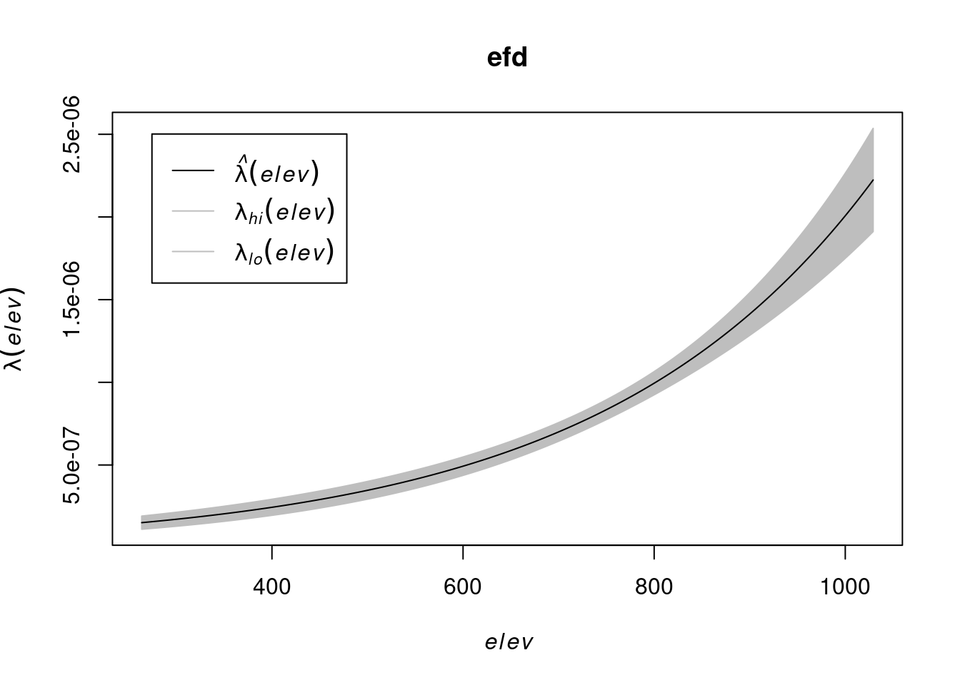
## Log intensity: ~elev
## Model depends on external covariate 'elev'
## Covariates provided:
##  elev: im
## 
## Fitted trend coefficients:
##   (Intercept)          elev 
## -16.629576223   0.003510778 
## 
##                  Estimate         S.E.       CI95.lo       CI95.hi Ztest
## (Intercept) -16.629576223 0.1944309612 -17.010653905 -16.248498542   ***
## elev          0.003510778 0.0002449191   0.003030746   0.003990811   ***
##                  Zval
## (Intercept) -85.52947
## elev         14.33444
## 
## ----------- gory details -----
## 
## Fitted regular parameters (theta):
##   (Intercept)          elev 
## -16.629576223   0.003510778 
## 
## Fitted exp(theta):
##  (Intercept)         elev 
## 5.996072e-08 1.003517e+00

Comparing models…

AIC(fit0)
## [1] 24535.8
AIC(fit1)
## [1] 24301.32

Model diagnostics…

diagnose.ppm(fit0)
diagnose.ppm(fit1)

## Model diagnostics (raw residuals)
## Diagnostics available:
##  four-panel plot
##  mark plot 
##  smoothed residual field
##  x cumulative residuals
##  y cumulative residuals
##  sum of all residuals
## sum of raw residuals in entire window = -8.035e-06
## area of entire window = 1.014e+09
## quadrature area = 1.011e+09
## range of smoothed field =  [-7.611e-07, 6.532e-06]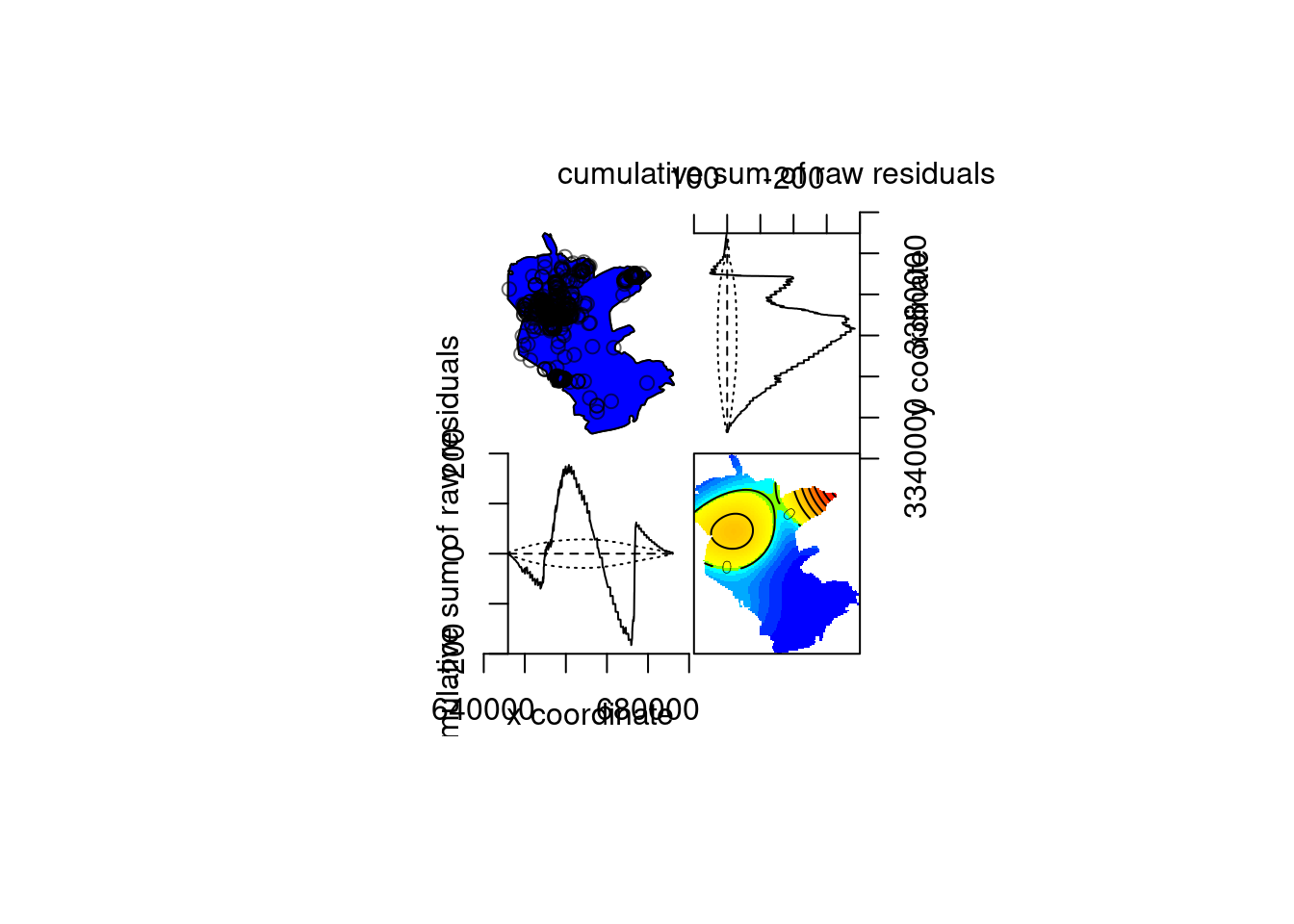

Figure 13.13: Model diagnostics

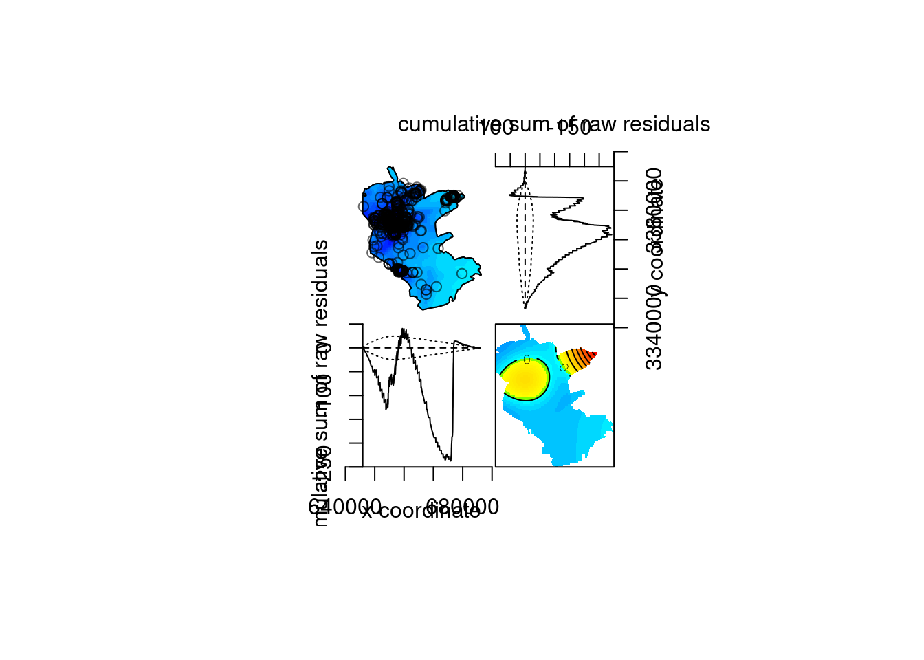
Figure 13.14: Model diagnostics

13.6.4 Effect function

efd = effectfun(
  fit1, 
  "elev", 
  visible = TRUE, 
  se.fit = TRUE
)

plot(efd)

13.6.5 Predictions

Predict…

pred0 = predict(fit0, elev)
pred1 = predict(fit1, elev)

Plot…

plot(pred0)

plot(pred1)